Note

This tutorial was generated from a Jupyter notebook that can be downloaded here.

Time evolution of starry maps

Warning

This tutorial showcases some experimental features. Modeling time evolution in starry is still quite clunky and inefficient. It is also extremely difficult! Whatever degeneracies we have in the static case (there are tons!) are made even worse by the fact that we now have many more degrees of freedom. Unless we have really good priors, it is very difficult to get meaningful results out of time-variable maps. We’re working on ways to make this easier, faster, and more tractable, so please stay tuned.

In this notebook, we’re going to take a look at how to model a star whose light curve evolves in time. The assumption here is that the evolution is due to either spot migration / evolution or differential rotation, so we need a way to model a time-variable surface map. There’s a few different ways we can do that. Please note that these are all experimental features – we’re still working on the most efficient way of modeling temporal variability, so stay tuned!

Let’s begin with our usual imports.

import matplotlib.pyplot as plt
import numpy as np
from tqdm.notebook import tqdm
from scipy.special import factorial
import starry

starry.config.lazy = False
starry.config.quiet = True

Generate the data

Let’s generate a map with three discrete Gaussian spots at different latitudes, rotating at slightly different rates due to a differential rotation with small shear \(\alpha = 0.02\). To create this dataset, we are linearly combining the flux generated from three separate maps and median-normalizing the light curve at the end.

We’re giving the map an inclination of 60 degrees and some limb darkening. These choices reduce the size of the null space slightly, making it easier to do inference. (Note that we are cheating since we assume below that we know the inclination and limb darkening exactly!)

inc = 60  # inclination
u1 = 0.5  # linear limb darkening coeff
alpha = 0.02  # differential rotation shear
P = 1.0  # equatorial period
intensity = -0.5  # spot intensity
sigma = 0.05  # spot size

# Generate a 10th degree map with linear limb darkening
np.random.seed(0)
map = starry.Map(10, 1)
map[1] = u1
omega_eq = 360.0 / P
time = np.linspace(0, 30, 1000)
time_ani = time[::10]
true_flux = np.zeros_like(time)
res = 300
true_image_rect = np.zeros((len(time_ani), res, res))
true_image_ortho = np.zeros((len(time), res, res))

# Generate light curves for three spots
true_lats = [-30, 30, -20]
true_lons = [-90, 60, 135]
for lat, lon in zip(true_lats, true_lons):

    # The angular velocity at the current latitude, computed
    # from the equation for linear differential rotation
    omega = omega_eq * (1 - alpha * np.sin(lat * np.pi / 180.0) ** 2)

    # Reset the map coefficients & add a new spot
    map.reset()
    map.inc = inc
    map[1] = u1
    map.add_spot(intensity=intensity, sigma=sigma, lat=lat, lon=lon)

    # Add to the flux
    true_flux += map.flux(theta=omega * time)

    # Add to our sky-prjected image
    true_image_ortho += map.render(theta=omega * time)

    # Hack: to get our lat-lon image, we need to manually
    # shift the image of each spot according to how far it
    # has lagged due to differential rotation. Sorry --
    # there's no easy way to do this in starry currently!
    tmp = map.render(projection="rect")
    shift = np.array((omega - omega_eq) * time_ani * res / 360, dtype=int)
    for n in range(len(time_ani)):
        true_image_rect[n] += np.roll(tmp, shift[n], axis=1)

# Normalize and add a little bit of noise
flux_err = 1e-5
flux = true_flux / np.nanmedian(true_flux)
flux += flux_err * np.random.randn(len(time))

We can visualize the map by passing in the image arrays. Let’s look at it in sky projection:

map.show(image=true_image_ortho, projection="ortho")

and in lat-lon coordinates that co-rotate with the equator (note that limb darkening is disabled in this projection by default):

map.show(image=true_image_rect, projection="rect")

Here’s the light curve we’re going to do inference on. You can tell there’s some differential rotation because of the change in the morphology over time:

plt.plot(time, true_flux / np.nanmedian(true_flux), "C0-", lw=1, alpha=0.5)
plt.plot(time, flux, "C0.", ms=3)
plt.gca().get_yaxis().get_major_formatter().set_useOffset(False)
plt.xlabel("time [days]")
plt.ylabel("flux [normalized]");

There are several ways to model this with starry, so let’s go over each one.

1. Using a Taylor expansion

Recall that in starry, the flux is a linear function of the spherical harmonic coefficient vector:

\[\mathbf{f} = \mathbf{A} \mathbf{x}\]

where \(\mathbf{f}\) is the flux vector, \(\mathbf{A} = \mathbf{A}(\Theta)\) is the design matrix (a function of a bunch of parameters \(\Theta\)) that transforms the map to a light curve, and

\[\mathbf{x} \equiv a \mathbf{y}\]

is the vector of spherical harmonic coefficients \(\mathbf{y}\) weighted by the map amplitude \(a\) (a value proportional to the luminosity of the map). If the map is time variable, we can express this by allowing \(\mathbf{x}\) to be a function of time: \(\mathbf{x} = \mathbf{x}(t) = a(t) \mathbf{y}(t)\). To make this tractable, we can Taylor expand this vector about \(t=0\):

\[\mathbf{x}(t) = \mathbf{x}\,\Big|_{t=0} \,\,\,+\,\,\, \mathbf{\dot{x}}\,\Big|_{t=0}t \,\,\,+\,\,\, \frac{1}{2}\mathbf{\ddot{x}}\,\Big|_{t=0}t^2 \,\,\,+\,\,\, ...\]

The corresponding flux vector (i.e., the light curve) is then

\[\mathbf{f} = \mathbf{A} \mathbf{x}\,\Big|_{t=0} \,\,\,+\,\,\, \mathbf{A} \mathbf{\dot{x}}\,\Big|_{t=0}t \,\,\,+\,\,\, \mathbf{A} \frac{1}{2}\mathbf{\ddot{x}}\,\Big|_{t=0}t^2 \,\,\,+\,\,\, ...\]

which we can write in matrix form as

\[\mathbf{f} = \mathbf{A'} \mathbf{x'}\]

where

\[\mathbf{A'} \equiv \Big( \mathbf{A} \quad \mathbf{A} t \quad \frac{1}{2} \mathbf{A} t^2 \quad ... \Big)\]

is an augmented design matrix and

\[\begin{split}\mathbf{x'} = \begin{pmatrix}\mathbf{x} \\ \mathbf{\dot{x}} \\ \mathbf{\ddot{x}} \\ ...\end{pmatrix}\end{split}\]

is the vector of spherical harmonic coefficients and their derivatives.

We can therefore linearly solve for the coefficients and their derivatives if we just augment the design matrix in this fashion (and provide suitable priors). Let’s do that below.

Let’s instantiate a map. We’ll solve for the map up to \(l = 5\) only and go up to 4th derivatives in the Taylor expansion. Note that we are solving for \(4 \times (5 + 1)^2 = 144\) coefficients in total, so we’ll need some good regularization to prevent overfitting.

map = starry.Map(5, 1)
map.inc = inc
map[1] = u1
order = 4

Here’s how to build the augmented design matrix:

# Compute the usual design matrix
theta = 360.0 / P * time
A0 = map.design_matrix(theta=theta)

# Normalize and center the time array
# (to help with numerical stability)
t = 2.0 * (time / time[-1] - 0.5)

# Horizontally stack the quantity 1/n! A0 t^n
coeff = 1.0 / factorial(np.arange(order + 1))
T = np.vander(t, order + 1, increasing=True) * coeff
A = np.hstack([(A0 * T[:, n].reshape(-1, 1)) for n in range(order + 1)])

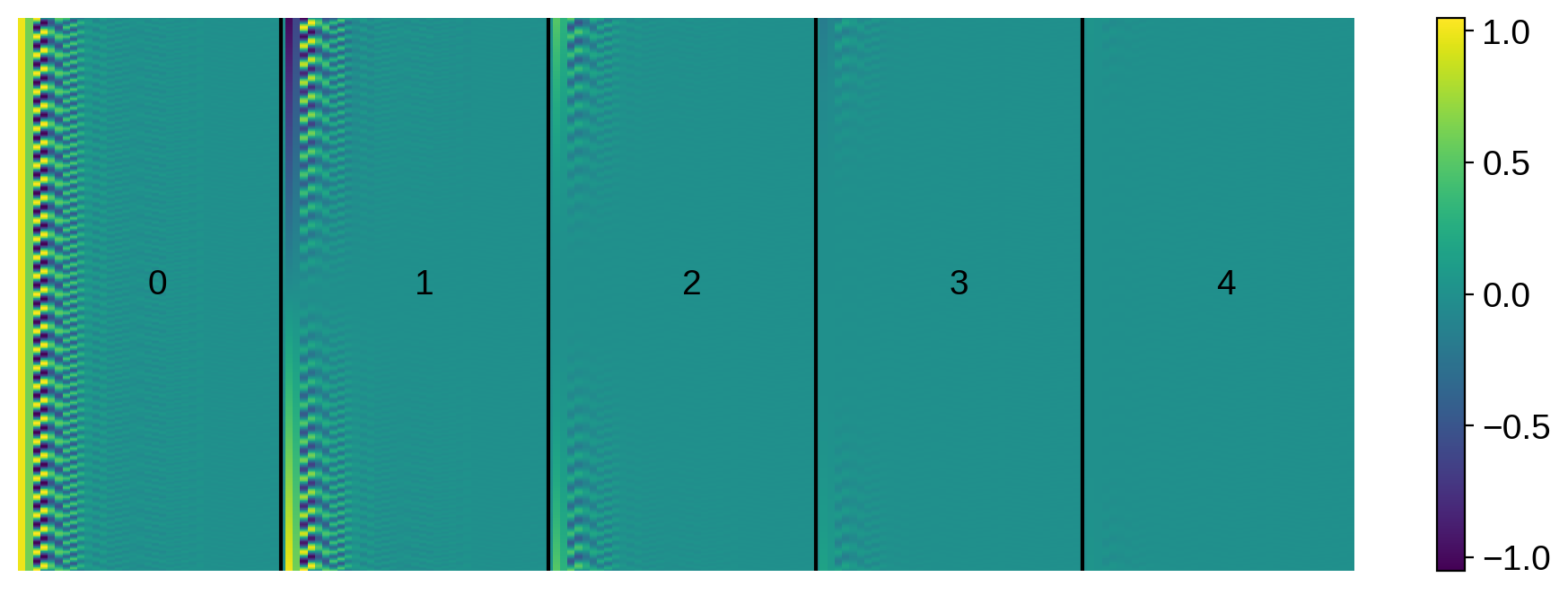
Here’s what that looks like (the derivative orders are indicated):

plt.imshow(A, aspect="auto")
[plt.axvline(n * map.Ny - 1, color="k") for n in range(1, order + 1)]
[
    plt.text(n * map.Ny - 1 + map.Ny / 2, len(t) / 2, n, color="k")
    for n in range(order + 1)
]
plt.gca().axis("off")
plt.colorbar();

Now we’ll tackle the linear problem.

Note

Since this is still an experimental feature, the user interface is a little clunky. Solving the linear problem for temporal maps will become easier in the next release of the code!

We’re going to use the solve method in the linalg module to solve a custom linear system. We’ll set the prior mean of the coefficients to zero, except for the first one, which we set to unity (since this is the prior on the map amplitude). We’ll give all the coefficients a prior variance of \(10^{-2}\), except for the first one, whose variance we’ll set to unity.

mu = np.zeros(A.shape[1])
mu[0] = 1.0
L = np.ones(map.Ny * (order + 1)) * 1e-2
L[0] = 1.0
x, cho_cov = starry.linalg.solve(A, flux, C=flux_err ** 2, mu=mu, L=L)

The solve method returns the amplitude-weighted coefficients x and the Cholesky factorization of the posterior covariance. Let’s plot the best fit model against the data:

model = A.dot(x)
plt.plot(time, flux, ".", ms=3, label="data")
plt.plot(time, model, label="model")
plt.ylabel("flux [normalized]")
plt.xlabel("time [days]")
plt.legend();

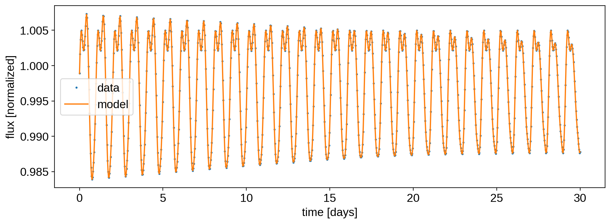
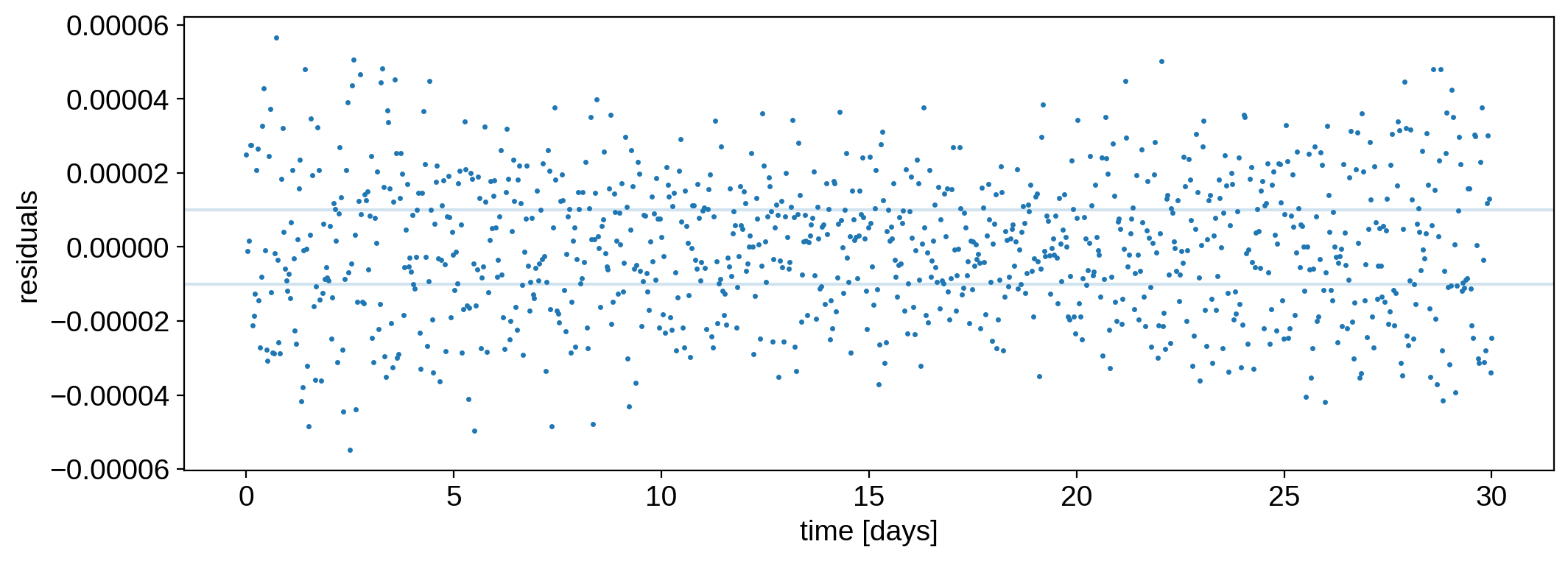
That looks really good! The residuals are fairly white:

plt.plot(time, flux - model, ".", ms=3, label="data")
plt.axhline(flux_err, color="C0", alpha=0.2)
plt.axhline(-flux_err, color="C0", alpha=0.2)
plt.ylabel("residuals")
plt.xlabel("time [days]");

Let’s now visualize the solution. Recall that the coefficients of the map at time \(t\) are given by

\[\mathbf{x}(t) = \mathbf{x}\,\Big|_{t=0} \,\,\,+\,\,\, \mathbf{\dot{x}}\,\Big|_{t=0}t \,\,\,+\,\,\, \frac{1}{2}\mathbf{\ddot{x}}\,\Big|_{t=0}t^2 \,\,\,+\,\,\, ...\]

# Allocate the image
image = np.empty((len(time_ani), res, res))

# Compute the weights of each coefficient in the Taylor expansion
t_ani = 2.0 * (time_ani / time_ani[-1] - 0.5)
T_ani = np.vander(t_ani, order + 1, increasing=True) * coeff

# At each point in time, compute the map coefficients
# and render the image
for n in range(len(time_ani)):
    xn = x.reshape(order + 1, -1).T.dot(T_ani[n])
    map.amp = xn[0]
    map[1:, :] = xn[1:] / map.amp
    image[n] = map.render(res=res, projection="rect")

map.show(image=image, projection="rect")
map.show(image=true_image_rect, projection="rect")

The posterior mean map is shown at the top and the original map is shown at the bottom. We’re able to recover the three spots and the general westward motion due to differential rotation, even though we never explicitly assumed anything about the number / shape / size of the spots or the strength of the differential rotation. There are, however, lots of artifacts in the solution, and one of the spots seems to disappear toward the end. They are also elongated latitudinally.

Note, however, that this is a fundamental limitation of the mapping problem, since the null space is huge! Unless we have good prior information, in many cases our maps will look nothing like the true image of the star.

2. Modeling differential rotation

Now let’s explicitly assume the variability we see is due to differential rotation. This is an experimental feature in starry, which you can read more about here. The idea is to Taylor expand the differential rotation operator and truncate the differentially-rotated map to the current map resolution. This is slow and becomes unstable as time goes on (since polynomials diverge toward infinity!) Below, we’re using a 2nd order expansion, which will help in modeling all 30 days of data at once. But it comes at the cost of extra computational overhead, so we’re going to again limit the map to a degree 5 spherical harmonic expansion.

Note

We’re still working on the differential rotation operator, so it will likely become a lot more efficient in the near future!

map = starry.Map(5, 1, drorder=2)
map.inc = inc
map.alpha = alpha
map[1] = u1

# Set the prior as before.
# We place a stronger prior on the coefficients
# to prevent the solution from blowing up (since
# the differential rotation operator isn't very
# numerically stable).
mu = np.zeros(map.Ny)
mu[0] = 1.0
L = np.ones(map.Ny) * 1e-4
L[0] = 1.0
map.set_prior(mu=mu, L=L)
map.set_data(flux, C=flux_err ** 2)

Center the array of rotational phases for numerical stability:

tmid = 0.5 * (time[-1] - time[0])
theta = 360.0 / P * (time - tmid)

Solve the linear problem (note that this automatically sets the map’s coefficients to the maximum a posteriori solution):

%%time
soln = map.solve(theta=theta)

CPU times: user 1.02 s, sys: 4.15 ms, total: 1.02 s
Wall time: 1.02 s

Compute and plot the model and the residuals:

%%time
model = map.flux(theta=theta)

CPU times: user 1.1 s, sys: 64 ms, total: 1.16 s
Wall time: 1.06 s

plt.plot(time, flux, ".", ms=3, label="data")
plt.plot(time, model, label="model")
plt.ylabel("flux [normalized]")
plt.xlabel("time [days]")
plt.legend();

plt.plot(time, flux - model, ".", ms=3, label="data")
plt.axhline(flux_err, color="C0", alpha=0.2)
plt.axhline(-flux_err, color="C0", alpha=0.2)
plt.ylabel("residuals")
plt.xlabel("time [days]");

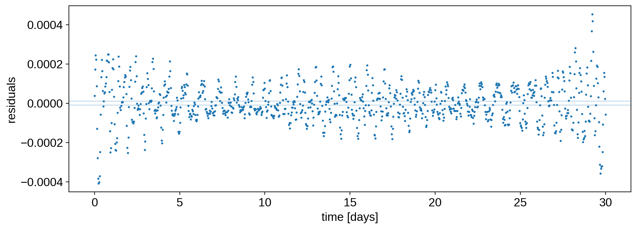
The fit is decent, but note how the scatter is much larger than the standard deviation of the data (blue lines).We’re also struggling to model the light curve at the edges of the timeseries. The oscillatory pattern in the residuals is due to the fact that our model assumes perfect differential rotation; i.e., that all features get sheared over time depending on their latitude. Our synthetic dataset consists of circular spots that move relative to each other, but don’t themselves undergo any shearing.

Here’s what the actual surface looks like:

map.show(theta=theta, projection="rect")
map.show(image=true_image_rect, projection="rect")

One could argue that there are three features in the solution that kind of track the true spots, but they’re shifted in latitude and elongated in longitude. They are also very prior-dependent (try experimenting with the value of \(\Lambda\)).

3. Spots rotating at different rates

Finally, we could place an even stronger prior on the problem and assume the stellar surface consists of a few discrete spots undergoing differential rotation.

Since the starry model is linear, we can instantiate several maps rotating at different rates, compute their light curves, and add them all together. We scale the result by the free variable scale to get the normalization correct.

We’re going to define a pymc3 model for the problem, but we’re not going to do any sampling – rather, we’re going to use the optimize function from exoplanet to find the best spot properties (and that requires a pymc3 model).

As we will see, finding the correct spot parameters is extremely difficult even when our model is exactly the correct description of the problem. That’s because the likelihood space is extremely degenerate and extremely multi-modal. Optimization yields completely different results depending on how exactly we initialize the solver and on how stringent our priors our. For simplicity, below we assume we know everything except for the latitude and longitude of each of the spots and the overall light curve normalization. We therefore fix the spot intensity, size, and differential rotation parameter at their true values. As we will see, even in this ideal case, we only get the correct solution if we initialize the solver very close to the true spot locations!

Warning

This next bit requires lazy evaluation mode. Switching between evaluation modes within a Python session is not currently supported. We do it below, but this is not advised in general, as it may lead to unexpected behavior.

# Switch evaluation modes.
# WARNING: Don't try this at home! Start a new Python session instead.
starry.config._lazy = True

Let’s define a function that instantiates a pymc3 model and runs an optimizer to find the spot locations. The function returns the best model for the light curve and for the image of the surface.

import pymc3 as pm
import exoplanet as xo


def solve(lat_guess, lon_guess):

    nspots = len(lat_guess)

    with pm.Model() as model:

        # Keep track of these things
        map = [None for n in range(nspots)]
        frac = [None for n in range(nspots)]
        flux_model = [None for n in range(nspots)]
        omega = [None for n in range(nspots)]

        # Flux normalization
        scale = pm.Uniform("scale", lower=0, upper=1.0, testval=1.0 / nspots)

        # Add each spot
        for n in range(nspots):

            # Spot parameters
            lat = pm.Uniform(
                "lat{}".format(n), lower=-90, upper=90, testval=lat_guess[n]
            )
            lon = pm.Uniform(
                "lon{}".format(n), lower=-180, upper=180, testval=lon_guess[n]
            )

            # Instantiate the map and add the spot
            map[n] = starry.Map(10, 1)
            map[n].inc = inc
            map[n][1] = u1
            map[n].add_spot(
                intensity=intensity, sigma=sigma, lat=lat, lon=lon,
            )
            omega[n] = omega_eq * (1 - alpha * np.sin(lat * np.pi / 180.0) ** 2)
            flux_model[n] = map[n].flux(theta=omega[n] * time)

        # Compute the model
        flux_model = scale * pm.math.sum(flux_model, axis=0)
        pm.Deterministic("flux_model", flux_model)

        # Save our initial guess
        flux_model_guess = xo.eval_in_model(flux_model)

        # The likelihood function
        pm.Normal("obs", mu=flux_model, sd=flux_err, observed=flux)

        # Optimize!
        map_soln = xo.optimize()

        # Render the map
        image = np.zeros((len(time_ani), res, res))
        for n in range(nspots):
            tmp = xo.eval_in_model(
                map[n].render(projection="rect", res=res), point=map_soln,
            )
            shift = np.array(
                (xo.eval_in_model(omega[n], point=map_soln) - omega_eq)
                * time_ani
                * res
                / 360,
                dtype=int,
            )
            for n in range(len(time_ani)):
                image[n] += np.roll(tmp, shift[n], axis=1)

    # Return the model for the flux and the map
    return map_soln["flux_model"], image

In our first experiment, we initialize the spot locations at random values centered on the true locations and with a standard deviation of 5 degrees. These are therefore very good guesses. Let’s see how we do:

np.random.seed(0)
lat_guess = true_lats + 5 * np.random.randn(3)
lon_guess = true_lons + 5 * np.random.randn(3)
model1, image1 = solve(lat_guess, lon_guess)

optimizing logp for variables: [lon2, lat2, lon1, lat1, lon0, lat0, scale]
105it [00:06, 15.97it/s, logp=1.009628e+04]
message: Desired error not necessarily achieved due to precision loss.
logp: -864216304.0448056 -> 10096.279660690363

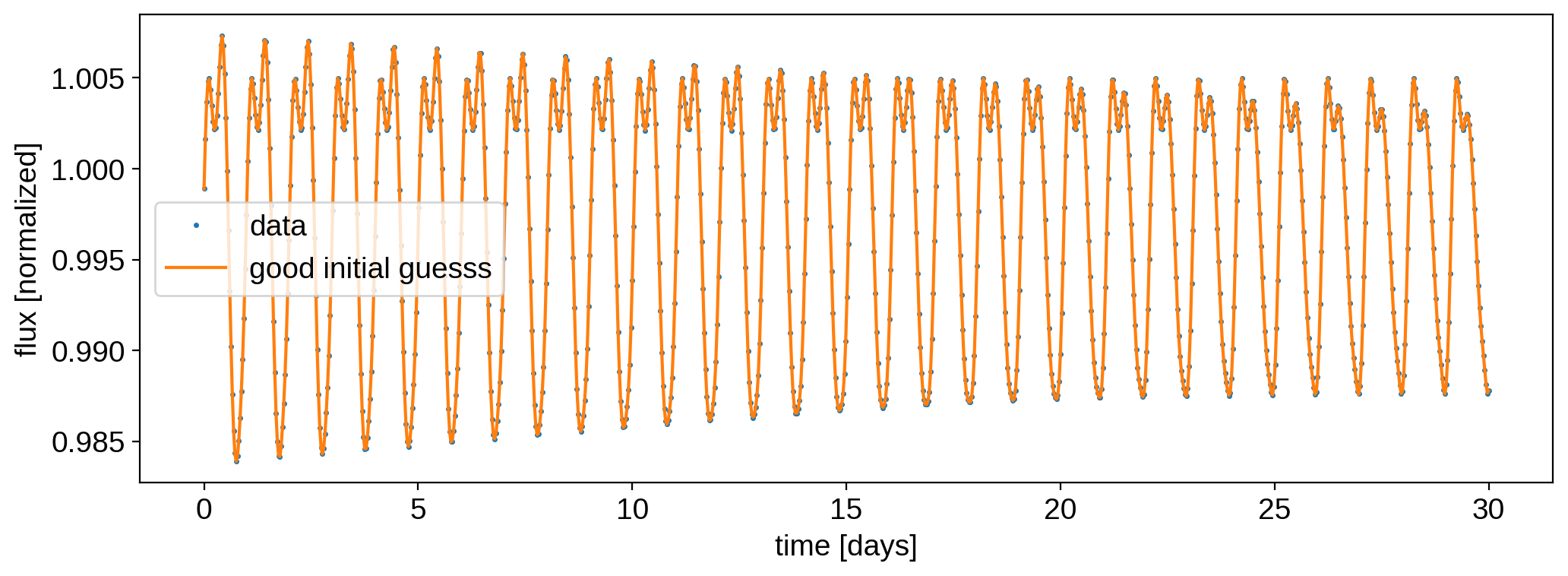
There was a huge improvement in the log likelihood! Here’s the final model and residuals:

plt.plot(time, flux, ".", ms=3, label="data")
plt.plot(time, model1, label="good initial guesss")
plt.ylabel("flux [normalized]")
plt.xlabel("time [days]")
plt.legend();

plt.plot(time, flux - model1, ".", ms=3, label="data")
plt.axhline(flux_err, color="C0", alpha=0.2)
plt.axhline(-flux_err, color="C0", alpha=0.2)
plt.ylabel("residuals")
plt.xlabel("time [days]");

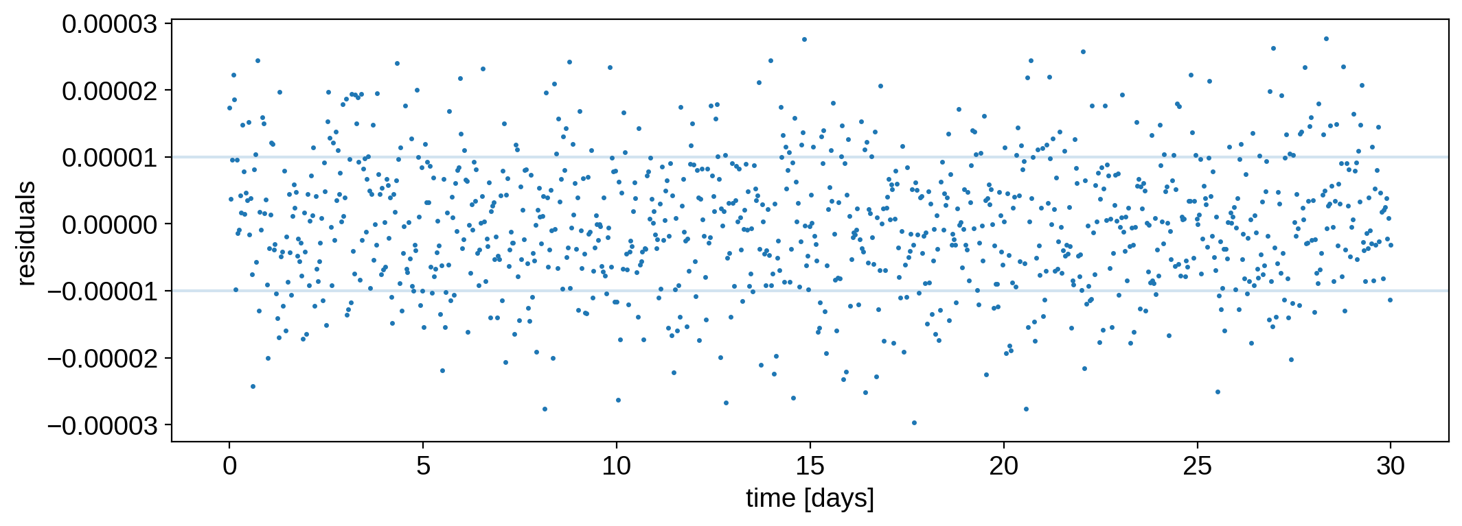
We have undoubtedly found the correct solution:

map.show(image=image1, projection="rect")
map.show(image=true_image_rect, projection="rect")

Now, to drive home the point of how difficult it is to model light curves with discrete spots, let’s instead initialize the solver with a slightly higher standard deviation in our guesses: 15 degrees:

np.random.seed(0)
lat_guess = true_lats + 15 * np.random.randn(3)
lon_guess = true_lons + 15 * np.random.randn(3)
model2, image2 = solve(lat_guess, lon_guess)

optimizing logp for variables: [lon2, lat2, lon1, lat1, lon0, lat0, scale]
135it [00:06, 21.54it/s, logp=-1.057833e+07]
message: Desired error not necessarily achieved due to precision loss.
logp: -1477879284.743772 -> -10578334.480908247

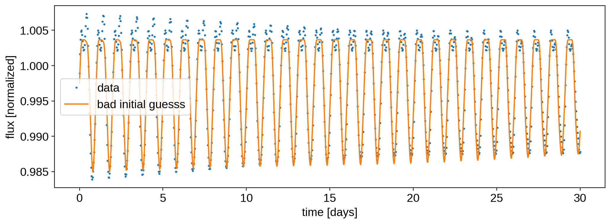
Note how our log likelihood is much, much smaller than before. Here’s the model:

plt.plot(time, flux, ".", ms=3, label="data")
plt.plot(time, model2, label="bad initial guesss")
plt.ylabel("flux [normalized]")
plt.xlabel("time [days]")
plt.legend();

plt.plot(time, flux - model2, ".", ms=3, label="data")
plt.axhline(flux_err, color="C0", alpha=0.2)
plt.axhline(-flux_err, color="C0", alpha=0.2)
plt.ylabel("residuals")
plt.xlabel("time [days]");

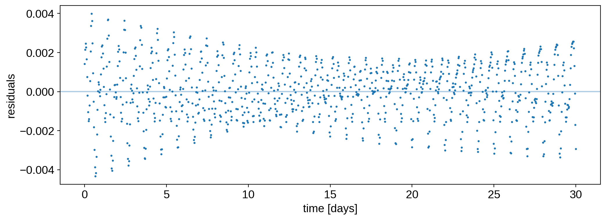
The residuals are orders of magnitude larger than the flux uncertainty. Check out the “best” map:

map.show(image=image2, projection="rect")
map.show(image=true_image_rect, projection="rect")

We clearly converged to a (very bad) local minimum that doesn’t even come close to describing the true surface of the star.

The bottom line here is that unless we have a very good initial guess (and/or a very good prior), it is really hard to do optimization in this space. However, if you’re patient, you could try initializing the solver at many different locations. You could also try optimizing for only a few variables at a time (for instance, solve for the position of the first spot with the other two fixed, then the position of the second spot with the other two fixed, and so forth), which sometimes helps with convergence. But that’s all beyond the scope of this simple tutorial.

Summary

We discussed three different methods to model time variability. Arguably none of them did particularly well. The discrete spot model got the correct solution when we fixed most of the parameters at their true values and started with a really good initial guess, but that’s hardly ever going to help us with real data. The differential rotation model was pretty meh and isn’t scalable to high degrees or long light curves because of how unstable the expansion of the differential rotation operator is. I’m a fan of the Taylor model, but it is quite ill-conditioned and therefore needs very strong priors to avoid overfitting. For real data, you should experiment with all three models, as some may perform better depending on the problem.

Kepp in mind that in all cases, the only way to get a good solution is to have a good prior (or a good initial guess). That’s because of the ever-present issue of the null space. The mapping problem is difficult enough when the maps are static, and becomes nearly intractable when there’s time variability.

However, there are many ways to maximize the information one can obtain about a stellar surface when there’s time variability, and they all rely on techniques to break degeneracies. Please refer to the null space tutorial for more information.