Note

This tutorial was generated from a Jupyter notebook that can be downloaded here.

Star spots

A major part of the philosophy of starry is a certain amount of agnosticism about what the surface of a star or planet actually looks like. Many codes fit stellar light curves by solving for the number, location, size, and contrast of star spots. This is usually fine if you know the stellar surface consists of a certain number of discrete star spots of a given shape. In general, however, that’s a very strong prior to assume. And even in cases where it holds, the problem is still extremely degenerate and lies in a space that is quite difficult to sample.

Instead, in starry we assume the surface is described by a vector of spherical harmonic coefficients. The advantage of this is that (1) it automatically bakes in a Gaussian-process smoothness prior over the surface map, in which the scale of features is dictated by the degree of the expansion; and (2) under gaussian priors and gaussian errors, the posterior over surface maps is analytic. If and only if the data and prior support the existence of discrete star spots on the surface, the posterior will reflect that.

However, sometimes it’s convenient to restrict ourselves to the case of discrete star spots. In starry, we therefore implement the add_spot method, which adds a spot-like feature to the surface by expanding a two-dimensional gaussian in terms of spherical harmonics.

Note

This method replaced the add_gaussian method in previous versions of the code.

In this notebook, we’ll take a look at how this new method works. For reference, here is the docstring of starry.Map.add_spot:

add_spot(amp=None, intensity=None, relative=True, sigma=0.1, lat=0.0, lon=0.0)

Add the expansion of a gaussian spot to the map.

This function adds a spot whose functional form is the spherical harmonic expansion of a gaussian in the quantity \(\cos\Delta\theta\), where \(\Delta\theta\) is the angular separation between the center of the spot and another point on the surface. The spot brightness is controlled by either the parameter amp, defined as the fractional change in the total luminosity of the object due to the spot, or the parameter intensity, defined as the fractional change in the intensity at the center of the spot.

Parameters

• amp (scalar or vector, optional) – The amplitude of the spot. This is equal to the fractional change in the luminosity of the map due to the spot. If the map has more than one wavelength bin, this must be a vector of length equal to the number of wavelength bins. Default is None. Either amp or intensity must be given.

• intensity (scalar or vector, optional) – The intensity of the spot. This is equal to the fractional change in the intensity of the map at the center of the spot. If the map has more than one wavelength bin, this must be a vector of length equal to the number of wavelength bins. Default is None. Either amp or intensity must be given.

• relative (bool, optional) – If True, computes the spot expansion assuming the fractional amp or intensity change is relative to the current map amplitude/intensity. If False, computes the spot expansion assuming the fractional change is relative to the original map amplitude/intensity (i.e., that of a featureless map). Defaults to True. Note that if True, adding two spots with the same values of amp or intensity will generally result in different intensities at their centers, since the first spot will have changed the map intensity everywhere! Defaults to True.

• sigma (scalar, optional) – The standard deviation of the gaussian. Defaults to 0.1.

• lat (scalar, optional) – The latitude of the spot in units of angle_unit. Defaults to 0.0.

• lon (scalar, optional) – The longitude of the spot in units of angle_unit. Defaults to 0.0.

Adding a simple spot

Let’s begin by importing stuff as usual:

import numpy as np
from scipy.integrate import dblquad
import starry

starry.config.lazy = False
starry.config.quiet = True

The first thing we’ll do is create a dummy featureless map, which we’ll use for comparisons below.

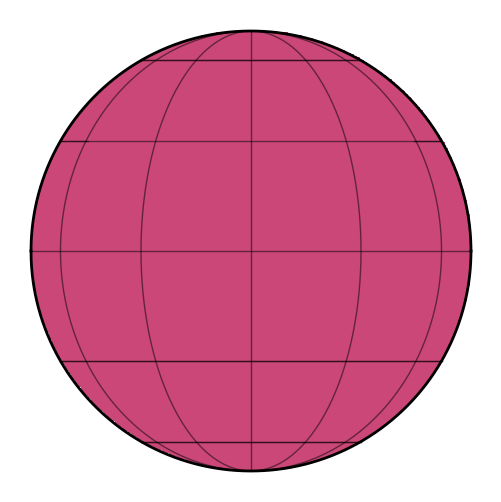
map0 = starry.Map(ydeg=1)
map0.show()

Now let’s instantiate a very high degree map and add a spot with an amplitude of \(1\%\) and a standard deviation of \(0.025\) at latitude/longitude \((0, 0)\):

amp = -0.01
sigma = 0.025
map = starry.Map(ydeg=30)
map.add_spot(amp=amp, sigma=sigma)

Here’s what we get:

map.show(theta=np.linspace(0, 360, 50))

The spot amplitude

Let’s take a look at what adding a spot does to the luminosity of a map. Recall that the integral of a quantity \(f\) over the surface of a sphere is given by \(\int_{0}^{2\pi}\int_{0}^{\pi}f\sin\theta\mathrm{d}\theta\mathrm{d}\phi\), where \(\theta\) is the polar angle (latitude plus \(\pi/2\)) and \(\phi\) is the longitude.

Let’s write a quick function to get the total luminosity of a starry map:

def integrand(theta, phi, map):
    lat = theta * 180 / np.pi - 90
    lon = phi * 180 / np.pi
    return map.intensity(lat=lat, lon=lon) * np.sin(theta)


def get_luminosity(map):
    res, _ = dblquad(
        integrand,
        0,
        2 * np.pi,
        lambda x: 0,
        lambda x: np.pi,
        epsabs=1e-4,
        epsrel=1e-4,
        args=(map,),
    )
    return res

As a baseline, let’s compute the total luminosity of the featureless map:

lum0 = get_luminosity(map0)
lum0

4.0

That may look weird, but this is actually how the normalization of spherical harmonic maps in starry is defined: they integrate to 4. The reason for this is rooted in the fact that the ratio between the projected area of a sphere (\(\pi r^2\)) and its total surface area (\(4\pi r^2\)) is equal to 4. If the total luminosity of a featureless map is 4, then the total flux seen from the object by any observer is unity:

map0.flux()

array([1.])

Since we usually normalize fluxes to unity, this made the most sense when defining the convention in starry. Note that in the general case, for a map with arbitrary surface features, the flux averaged over all observers is unity.

Anyways, let’s compute the luminosity of the map with the spot on it. So we don’t need to worry about the normalization, let’s compute it as a fraction of the luminosity of the featureless map:

lum = get_luminosity(map)
lum / lum0

0.9900000014159245

As promised, the spot decreased the total luminosity of the map by one percent!

The spot intensity

Instead of specifying the spot amplitude, we can specify the spot intensity. This is the fractional change in the intensity of the map at the center of the spot. Let’s give the spot an intensity of 10 percent:

intensity = -0.1
sigma = 0.025
map = starry.Map(ydeg=30)
map.add_spot(intensity=intensity, sigma=sigma)

map.show(theta=np.linspace(0, 360, 50))

We can plot the intensity along the equator:

lon = np.linspace(-90, 90, 100)
plt.plot(lon, map.intensity(lon=lon) / map0.intensity())
plt.xlabel("longitude [deg]")
plt.ylabel("intensity");

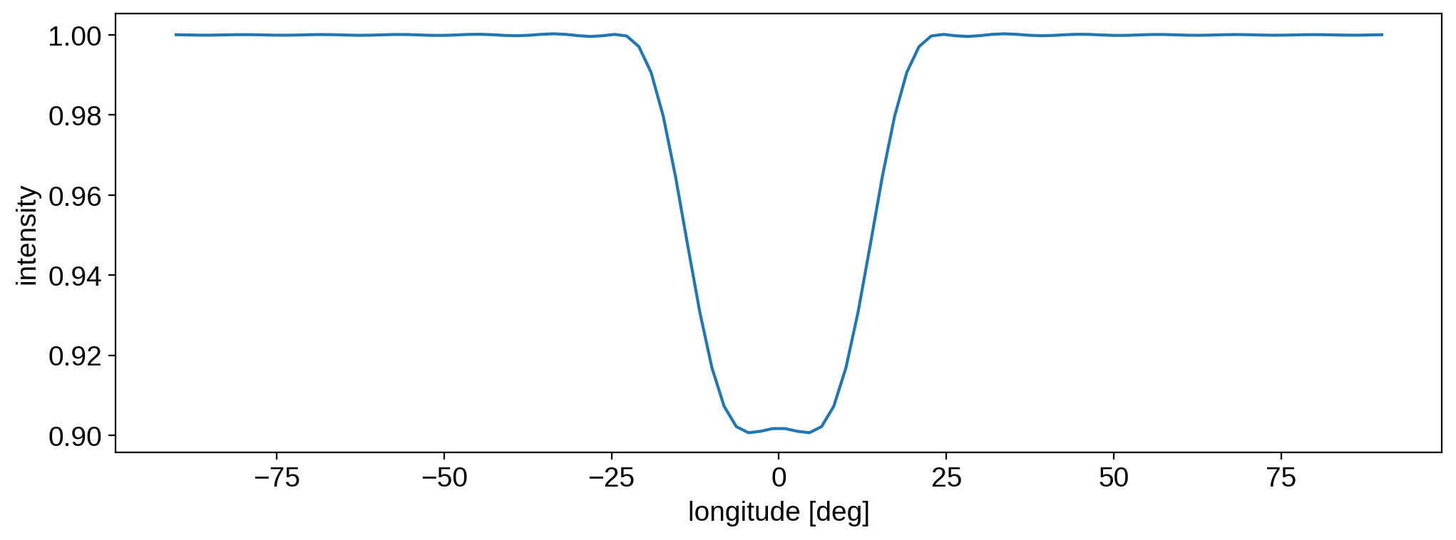
It’s clear that the intensity at the center of the spot is \(90\%\) that of the unspotted map.

Just for fun, let’s compute the total luminosity:

lum = get_luminosity(map)
lum / lum0

0.998433192469363

The luminosity has decreased, but only by about one tenth of a percent.

Note

As we will see below, the spot generated by starry is a Taylor expansion of a gaussian. The relationship between the spot amplitude and its intensity is computed for the actual gaussian, so for low degree maps there may be some disagreement between (say) the intensity the user specifies and the actual intensity at the center of the spot.

The spot expansion

As mentioned in the docstring, the spot is modeled as a gaussian in \(\cos(\Delta\theta)\), where \(\Delta\theta\) is the angular distance on the surface of the body. Let’s verify this by plotting the intensity of our star as a function of longitude along the equator and comparing it to that of a gaussian:

# Compute the intensity along the equator
# Remove the baseline intensity and normalize it
lon = np.linspace(-90, 90, 100)
baseline = 1.0 / np.pi
I = -(map.intensity(lon=lon) - baseline) / (map.intensity(lon=0) - baseline)

# Compute the intensity of a normalized gaussian
# in cos(longitude) with the same standard deviation
coslon = np.cos(lon * np.pi / 180)
I_gaussian = -np.exp(-((coslon - 1) ** 2) / (2 * sigma ** 2))

# Compare the two
plt.plot(lon, I, label="starry ($l = 30$)")
plt.plot(lon, I_gaussian, label="gaussian")
plt.legend()
plt.xlabel("longitude [deg]")
plt.ylabel("normalized intensity");

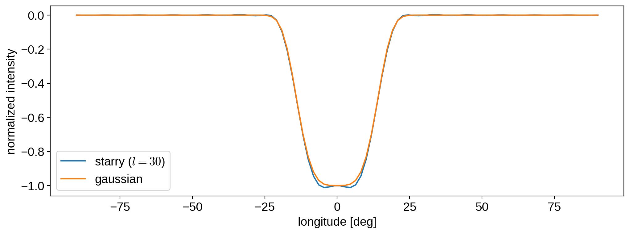
The expressions agree quite well. However, keep in mind that the spot is still only an approximation to a gaussian; it is, in fact, the two-dimensional Taylor expansion of a gaussian on the sphere. You can see that there are small wiggles in the blue curve, which will become more pronounced the smaller the spot size \(\sigma\) or the smaller the spherical harmonic degree of the expansion. Consider this same plot, but for a map of degree 15 instead of 30:

map15 = starry.Map(ydeg=15)
map15.add_spot(amp, sigma=sigma)
I15 = -(map15.intensity(lon=lon) - baseline) / (map15.intensity(lon=0) - baseline)

plt.plot(lon, I15, label=r"starry ($l = 15$)")
plt.plot(lon, I_gaussian, label="gaussian")
plt.legend()
plt.xlabel("longitude [deg]")
plt.ylabel("normalized intensity");

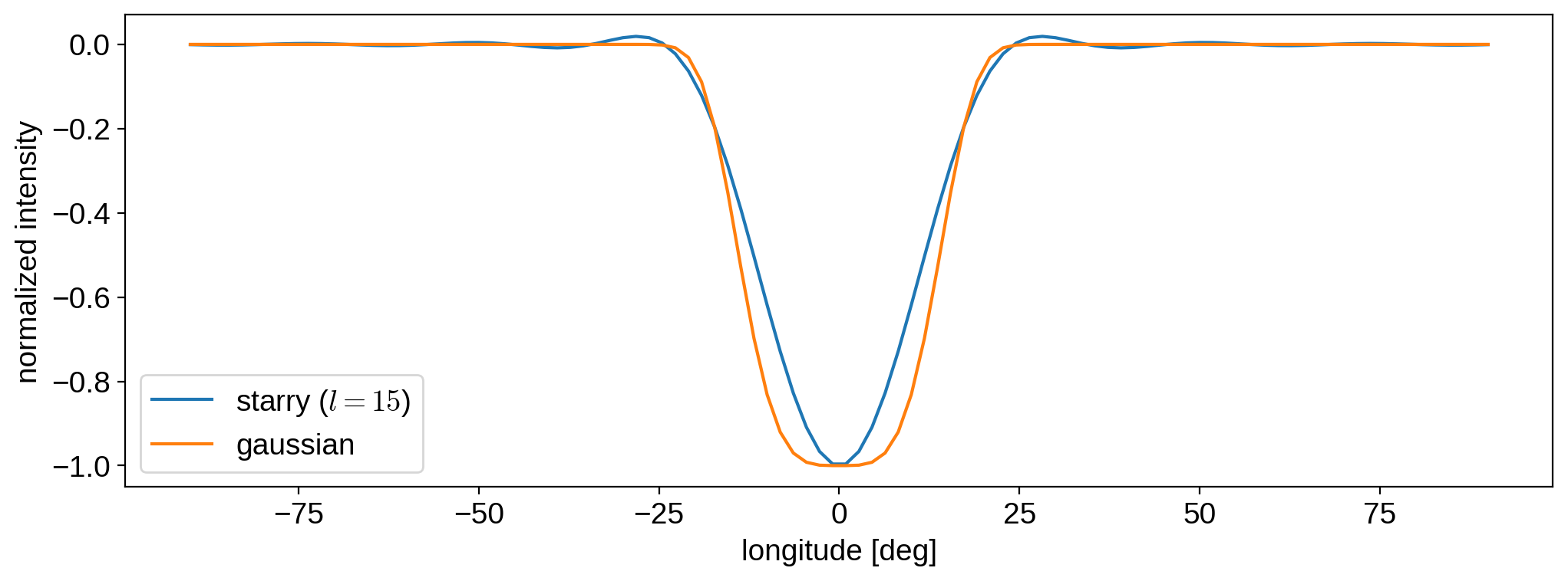
Here, the oscillations are far more evident. In general, users should be careful when trying to model small spots with low-\(l\) expansions. It’s always useful to plot the intensity, or even just visualize the map, to ensure that the degree of the map is high enough to resolve the size of the spots.