Note

This tutorial was generated from a Jupyter notebook that can be downloaded here.

Maps in reflected light

This notebook discusses how to model light curves in reflected light. Currently, starry can only model phase curves in reflected light, since the math behind occultation light curves is a bit trickier (we’re working on it, though, so stay tuned!) Additionally, starry computes illumination profiles assuming the distance between the illumination source and the body is large; i.e., the illumination source is effectively a point source. This will also likely be relaxed in a future release.

Let’s begin by instantiating a map in reflected light. We do this by specifying reflected=True when calling starry.Map().

import matplotlib.pyplot as plt
import numpy as np
import starry

starry.config.lazy = False
starry.config.quiet = True

map = starry.Map(ydeg=15, reflected=True)

Before we set any spherical harmonic coefficients, let’s take a look at our map. We can call the show() method as usual:

map.show()

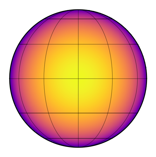
By default, the illumination source is along the \(+\hat{z}\) direction, so directly in front of the object. You can tell that points in the center of the map (where it is noon) are brighter than points along the edges (where it is dawn or dusk). To change the location of the illumination source, we edit the xs, ys, and zs keywords, just as we do when calling the flux() method. These are the Cartesian coordinates of the illumination source.

map.show(xs=1, ys=0, zs=0)

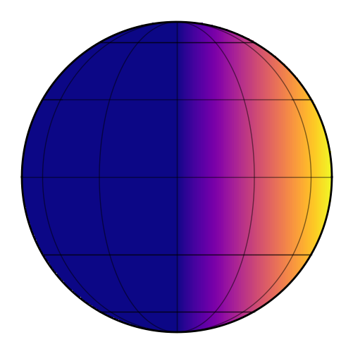
We are now viewing a uniform map illuminated from the side. The intensity on the left half is zero, since it is completely unilluminated.

The distance between the body and the source, \(r = \sqrt{x_s^2 + y_s^2 + z_s^2}\), controls the overall amplitude of the flux. We can check that it follows the expected one-over-r-squared law:

r = np.logspace(-1, 2)
plt.figure(figsize=(12, 5))
plt.plot(r, map.flux(xs=0, ys=0, zs=r), label="flux")
plt.plot(r, 1 / r ** 2, label=r"$1/r^2$", ls="--")
plt.plot(1, 1, "ko")
plt.axvline(1, color="k", ls="--", lw=1, alpha=0.5)
plt.axhline(1, color="k", ls="--", lw=1, alpha=0.5)
plt.yscale("log")
plt.xscale("log")
plt.legend(fontsize=18)
plt.xlabel("distance", fontsize=24)
plt.ylabel("flux", fontsize=24);

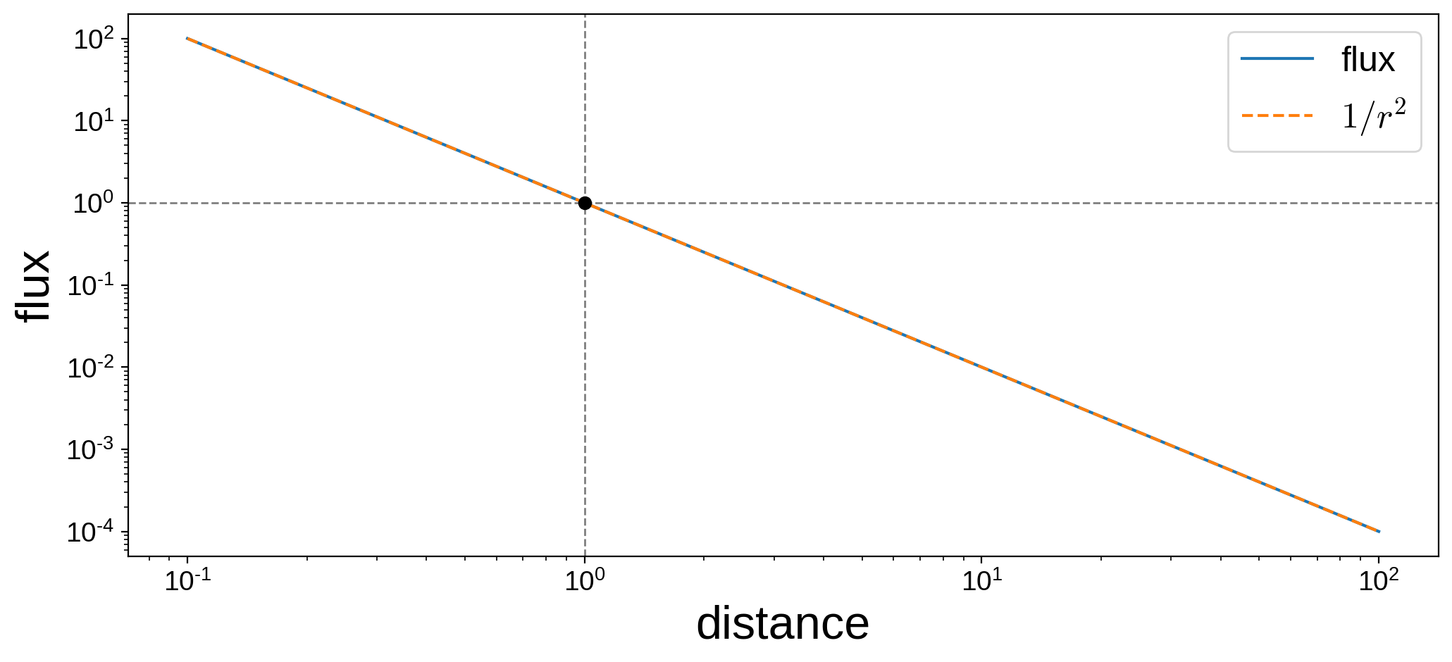
In particular, note that the flux in starry is normalized such that when the distance between the occultor and the illumination source is unity, a uniform unit-amplitude map illumminated by a unit-amplitude source will emit a flux of unity when viewed at noon.

Moving on, reflected light maps behave exactly like regular spherical harmonic maps, except the spherical harmonic coefficients y represent the expansion of the surface albedo rather than emissivity. Let’s load the continental map of the Earth and give the map the same obliquity as the Earth:

map.load("earth", sigma=0.075)
map.obl = 23.5

Let’s view the half-Earth rotating over one cycle:

map.show(theta=np.linspace(0, 360, 50), xs=1, ys=0, zs=0)

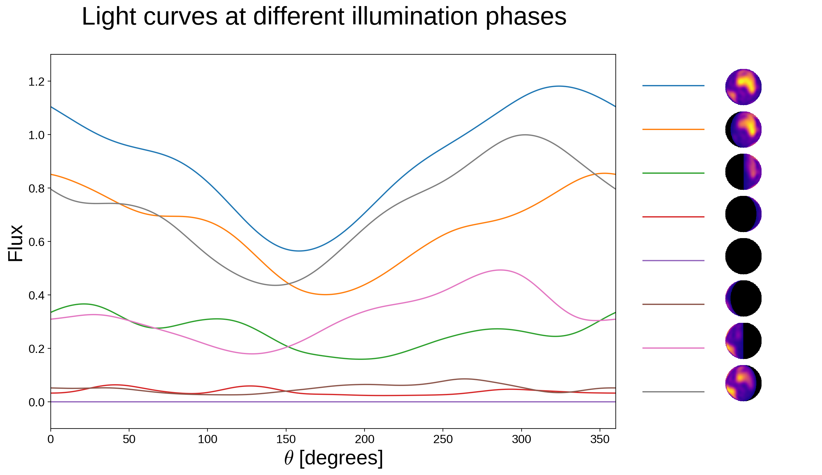
The above animation corresponds to the (northern) winter solstice. Here’s the phase curve of the Earth over one rotation at 8 different illumination phases:

fig = plt.figure(figsize=(12, 8))
theta = np.linspace(0, 360, 1000)
phis = np.linspace(0, 360, 9)[:-1]
xs = np.cos((phis - 90) * np.pi / 180)
zs = -np.sin((phis - 90) * np.pi / 180)
for n, phi in enumerate(phis):
    plt.plot(theta, map.flux(theta=theta, xs=xs[n], ys=0, zs=zs[n]), label=phi)
plt.xlim(0, 360)
plt.ylim(-0.1, 1.3)
plt.xlabel(r"$\theta$ [degrees]", fontsize=24)
plt.ylabel("Flux", fontsize=24)
legend = plt.legend(
    loc="center left", bbox_to_anchor=(1, 0.5), fontsize=36, frameon=False
)
for text in legend.get_texts():
    text.set_color("w")
cmap = plt.get_cmap("plasma")
cmap.set_under("#000000")
for n in range(8):
    ax = fig.add_axes((1.05, 0.775 - 0.087 * n, 0.05, 0.075))
    img = map.render(res=100, xs=xs[n], ys=0, zs=zs[n])
    ax.imshow(img, cmap=cmap, origin="lower", vmin=1e-5, vmax=1.0)
    ax.axis("off")
plt.suptitle("Light curves at different illumination phases", fontsize=30);

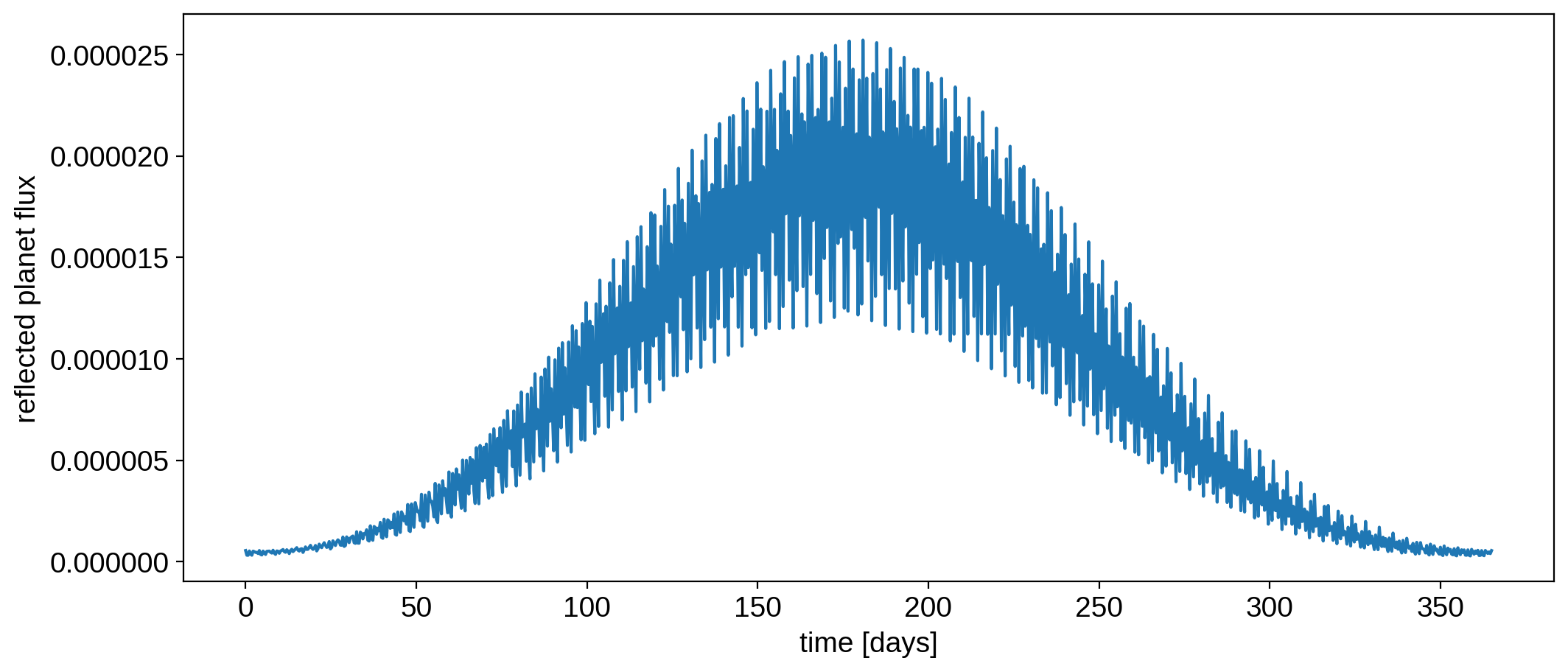
And here’s the phase curve of the Earth over one year in orbit around the Sun:

sun = starry.Primary(starry.Map())
earth = starry.Secondary(map, porb=365.0, prot=1.0, m=0.0, inc=60)
earth.map.inc = earth.inc = 60
sys = starry.System(sun, earth)

t = np.linspace(0, 365.0, 1000)
plt.figure(figsize=(12, 5))
plt.plot(t, sys.flux(t, total=False)[1])
plt.xlabel("time [days]")
plt.ylabel("reflected planet flux");