Note

This tutorial was generated from a Jupyter notebook that can be downloaded here.

Warning

This tutorial showcases an experimental feature. The way starry models differential rotation is likely to change in the future. We’re working on making it faster and better conditioned for large values of alpha.

Differential Rotation

The new version of starry implements an experimental version of differential rotation. This is still an experimental feature, mostly because it is extremely slow to compute. Because differential rotation leads to winding of features on the surface, the angular scale of these surface features becomes smaller and smaller with time, so the actual degree of the spherical harmonic expansion we’d need to preserve these features would increase without bound. starry implements a truncated expansion of the effect of differential rotation, but the operations still scale very steeply with the degree of the original map. Additionally, the approximation becomes worse and worse over time. This is something fundamental about differential rotation: it’s simply not possible to model it accurately with spherical harmonics.

However, for weak differential rotation (\(\alpha \ll 1\)) and over short timescales, the implementation in starry may still be useful! Let’s take a look.

Let’s import starry as usual, and disable lazy evaluation.

import starry
import numpy as np
import matplotlib.pyplot as plt

starry.config.lazy = False
starry.config.quiet = True

To create a map with differential rotation enabled, pass the drorder keyword to starry.Map(). This is the order of the approximation to differential rotation and should usually be 1 (or 2 if absolutely necessary). In general, the spherical harmonic expansion scales terribly with the order.

map = starry.Map(ydeg=5, drorder=1)

Let’s incline the map a bit and give it a dipole-like feature:

map.inc = 60
map[2, 0] = 1

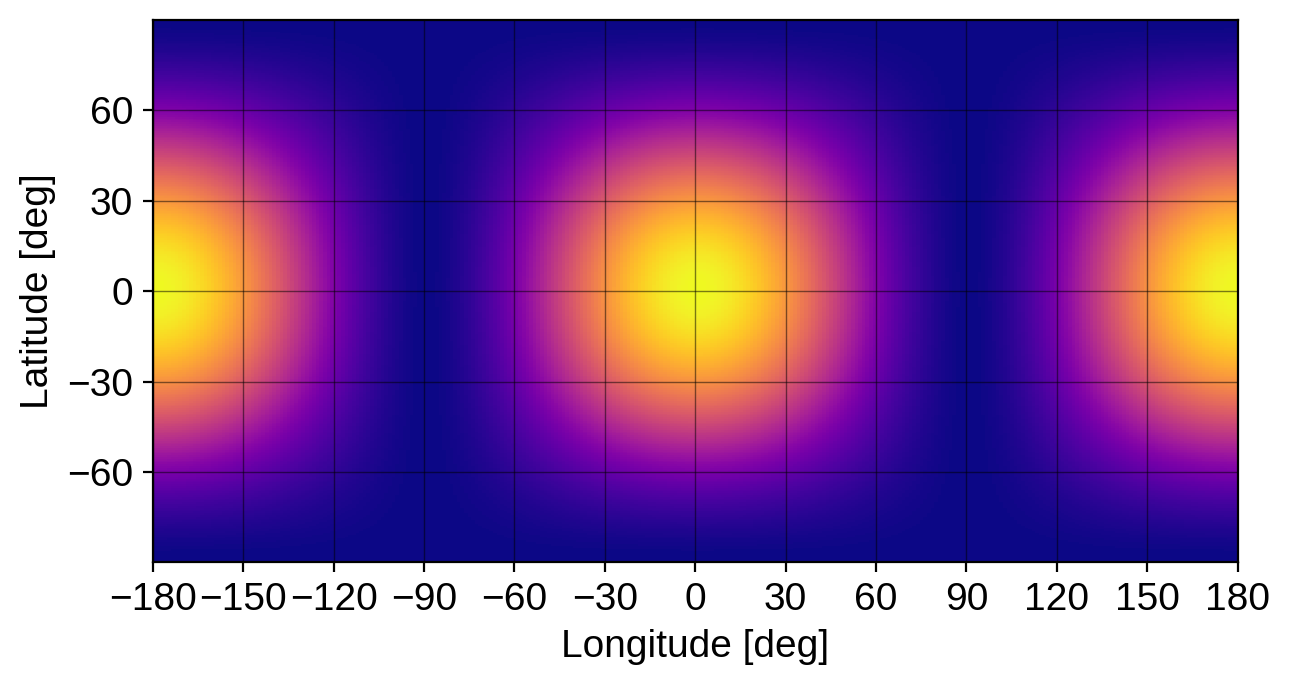
Here’s what that looks like in lat-lon coordinates:

map.show(projection="rect")

And here’s an animation over two rotation cycles (no differential rotation yet):

map.show(theta=np.linspace(0, 720, 200), dpi=150)

and the corresponding light curve:

theta = np.linspace(0, 720, 1000)
flux0 = map.flux(theta=theta)
plt.plot(theta, flux0);

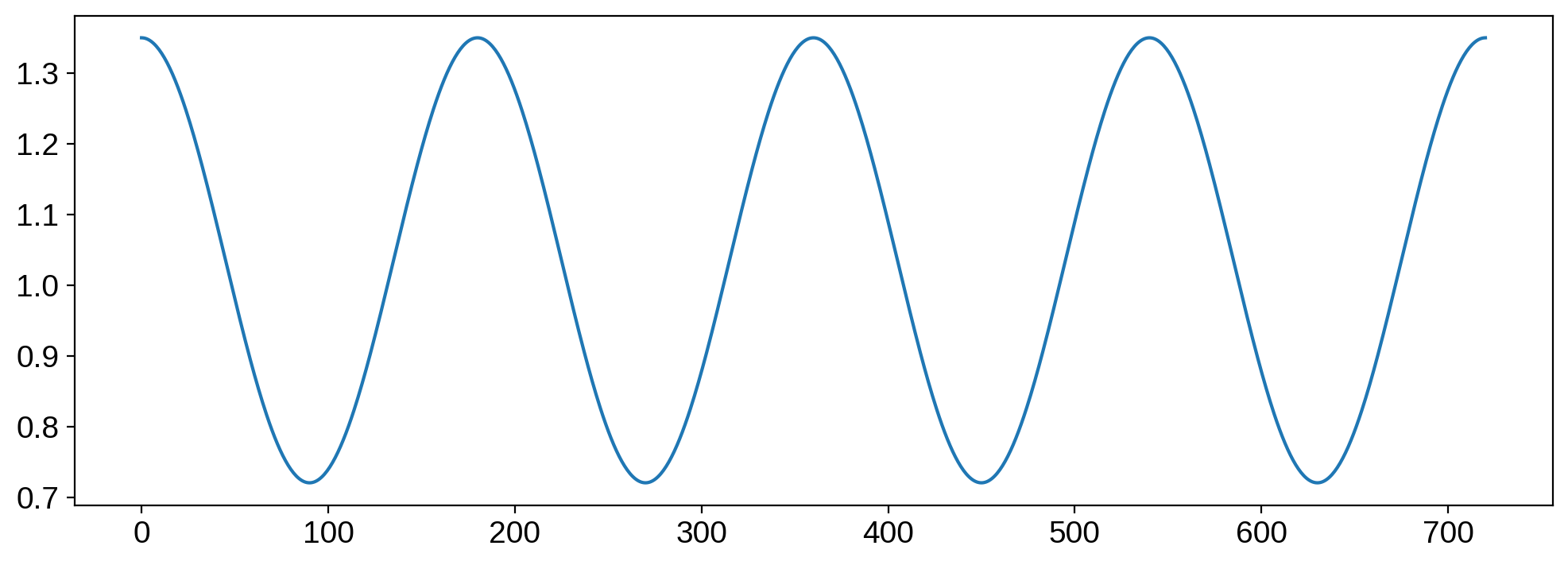
We haven’t yet provided a value for the differential rotation parameter, so there’s nothing exciting going on. To do that, we specify the \(\alpha\) parameter, which is the linear shear due to differential rotation:

map.alpha = 0.1

Given this linear shear, the angular velocity \(\omega\) at a latitude \(\phi\) on the surface is given by

\(\omega(\phi) = \omega_{eq}(1 - \alpha \sin^2\phi)\),

where \(\omega_{eq}\) is the angular velocity at the equator.

Here’s what the rotating map now looks like over two cycles. Note the shearing away from the equator:

map.show(projection="rect", theta=np.linspace(0, 720, 100))

Here’s the same map in projection:

map.show(theta=np.linspace(0, 720, 200), dpi=150)

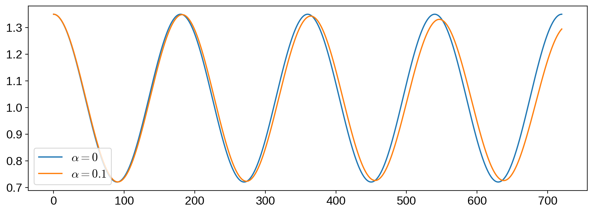
Finally, let’s compare the two light curves:

theta = np.linspace(0, 720, 1000)
flux = map.flux(theta=theta)
plt.plot(theta, flux0, label=r"$\alpha = 0$")
plt.plot(theta, flux, label=r"$\alpha = 0.1$")
plt.legend(loc="lower left");

Finally, another word of caution. Since differential rotation leads to increasingly smaller features on the surface, the starry approximation breaks down after a certain amount of time. The plots below show images of the surface of this star for different values of the quantity \(\omega t \alpha\), in which the expansion is done in starry.

Note that for small values of \(\omega t \alpha\), things look great, but above about \(90^\circ\), the polar regions develop unphysical “blobs”. That’s the limited resolution of the map kicking in: there’s no easy way to accurately describe a strongly sheared profile with \(l = 5\) spherical harmonics!

The blue and orange lines show the position of the peak intensity of the map, computed analytically (blue) and from the starry approximation (orange). The starry solution tracks the analytic one pretty well also up to about \(90^\circ\), beyond which the limiations of the approximation becomes evident.

So, bottom line: when drorder=1, the starry approximation is only good up to about \(\omega t \alpha = 90^\circ\).