
Synthetic Likelihoods
In this post I dig a little deeper into the assumptions I'm making when I try to model stellar surfaces (and, equivalently, stellar light curves) using a Gaussian Process. The true likelihood function for the data is certainly not a gaussian, but it turns out that approximating it as such is not a terrible idea. Here I'll discuss the concept of a synthetic likelihood, which is a term from the ecology literature (and is probably called different things in different fields), and explore its behavior with a very simple toy model. I'll warn you right now that I'm in a bit over my head with this, so comments / thoughts from proper statisticians are most welcome!
Difficult Integrals
Thanks to its applications in the machine learning community, variational inference (VI) is now a popular method to approximate posterior distributions when the true density is difficult to compute. Rather than compute the posterior by sampling (such as in Markov Chain Monte Carlo), VI approximates the posterior via optimization. In the simplest variant of the method, one assumes the posterior distribution can be approximated by a (multivariate) gaussian and runs VI to find the mean(s) and variance(s) of the gaussian that best matches the true posterior. This is typically done by minimizing the K-L divergence between the two distributions. VI can be an excellent choice for otherwise intractable problems, but it does have drawbacks: in its vanilla form it is unable to capture multi-modality and can underestimate the posterior variance in the presence of correlated parameters.
In my research on modeling stellar light curve variability the posterior distributions I'm interested in are often very intractable. Not because they're inherently difficult to sample from, but because my likelihood function is so difficult to compute. Briefly, I'm interested in inferring star spot properties, such as their typical sizes and latitudes, from stellar light curves. This is a notoriously ill-posed problem (Basri et al. 2020 is a nice review), as there are perfect degeneracies at play that can lead to an infinite number of equally likely surface map solutions for a given light curve. As I described in previous blog posts, one trick is to accept that we cannot know exactly what any stellar surface looks like and instead directly solve for the statistics we care about: the distribution of star spot sizes and latitudes, irrespective of how big any individual spot is or where it is on the star. This works even better if we have an ensemble of light curves of "similar" stars: we can use their collective information to better constrain the statistics of star spots across all members of the ensemble.
This is all well and good until we think about the integrals we need to compute along the way. What I described above was the process of marginalizing over the nuisance parameters (the nitty gritty details of individual spots) to compute the marginal likelihood that a given star (or a given ensemble of stars) is a draw from a particular distribution of star spot sizes and latitudes.
Say we have some set of parameters $\theta$ controlling the spot distributions (say, the mean and variance of the spot size distribution, the mean and variance of the spot latitude distribution, etc.) The marginal likelihood is the probability of our data $y$ given $\theta$, which can be computed by integrating over all the nuisance parameters $c_0 \, \cdots \, c_n$:
$$p\big(y \, \big| \, \theta \big) = \int \, \cdots \, \int p\big(y \, \big| \, c_0 \, \cdots \, c_n\big) p\big(c_0 \, \big| \, \theta\big) \mathrm{d}c_0 \, \cdots \, p\big(c_n \, \big| \, \theta\big) \mathrm{d}c_n$$
Computing this is a tall order, especially since $n$ can be quite large (hundreds or even thousands in my problems). Instead of attempting to solve this integral exactly, the approach I took was to assume that my marginal likelihood can be well approximated by a multidimensional gaussian (see this blog post). The task then is to find how its mean $\mu(\theta)$ and the covariance $\Sigma(\theta)$ depend on the parameters I care about, $\theta$.
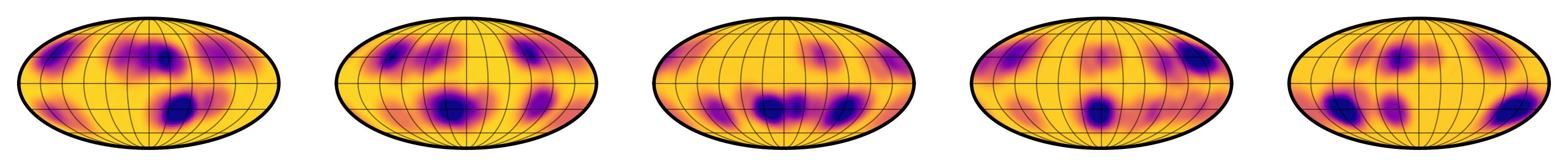
Figure 1 Random samples from the true distribution of star spots conditioned on a specific value of $\theta$, a vector that includes (among other things) the spot size distribution mean and variance and the spot latitude distribution mean and variance.
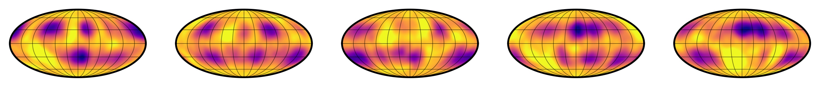
Figure 2 Random samples from the multidimensional gaussian approximation to the distribution in Figure 1.
This is where I thought about the parallels to variational inference, since again we're doing some sort of optimization to find the gaussian that best describes our probability distribution. Here, however, I am computing the variational distribution for the likelihood, not the posterior. So this isn't really VI at all! I spent a while poking around online to figure out what exactly the name for what I was doing was, and I found several papers in ecology doing similar things. They all date back to this paper by Wood (2010), who developed an approach he dubbed the synthetic likelihood.
The Synthetic Likelihood
The idea is fairly straightforward. The data consists of measurements of the size of an insect population over time, and the ecologist's task is to infer some fundamental parameter of the population that controls its growth rate. The problem is that the process generating the data is extremely chaotic; the population undergoes sudden, fast, and unpredictable jumps and declines in size due to various random environmental pressures. Thus, basic aspects of the dataset such as the particular times at which these spikes occur are mostly random and thus unrelated to the true parameters we care about. However, statistics of the dataset (such as, perhaps, the frequency of spikes, their relative amplitudes, the details of the shape of the spikes, etc.) are informative.
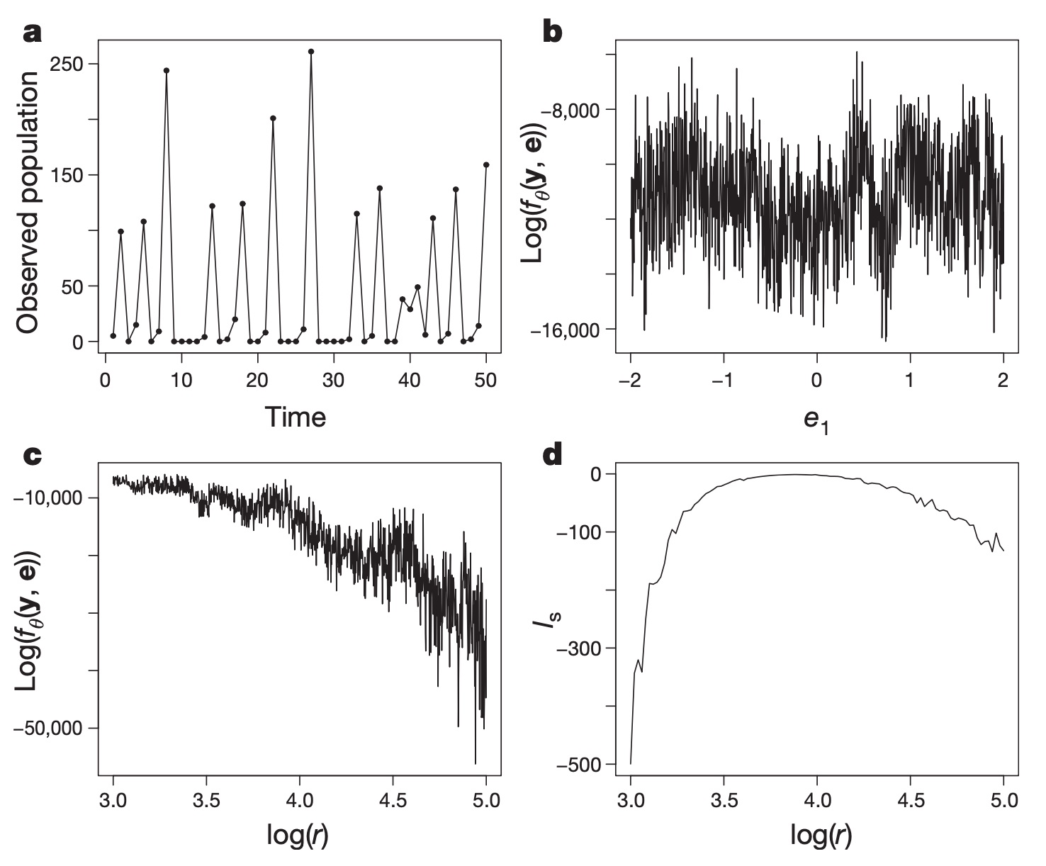
Figure 3 Reproduction of Figure 1 in Wood (2010). Panel a is the data: the size of the population over time. Panels b and c are the log likelihood as a function of a noise parameter $e_1$ and the growth rate parameter $r$, conditioned on the true values of $r$ and $e_1$, respectively. In addition to being difficult to compute, this likelihood is extremely noisy. Panel d is the (marginal) log synthetic likelihood, which is much smoother and peaks close to the true value $\log r = 3.8$.
The thing to do is therefore compute the likelihood marginalized over the phase of the spikes: that is, integrating over all of the (infinite number of) ways in which a population with a given intrinsic growth rate $r$ can evolve under a chaotic noise process. This is the same intractable integral as in the star spot mapping problem! In Wood's case, he needs to marginalize over the phases of the population spikes; in my case, I need to marginalize over the phases of the spots (among other things).
Wood's approach to computing this intractable integral is to bypass it by sampling. Chaotic systems are easy enough to forward model: pick a value of $r$, pick some parameters of the noise process, set your initial conditions, and diff-eq away. For a fixed value of $r$, we can generate lots (say, hundreds of thousands) of synthetic datasets. Each one will have spikes in different places and look different overall, but they will all be draws from the exact same statistical process. The trick then is to compute the empirical mean and (dense) covariance matrix from this simulated dataset, compute the likelihood of the corresponding gaussian, and call it a day. He dubs this likelihood function the synthetic likelihood.
Wood goes on to show just how powerful this approximate inference technique is in modeling chaotic ecological systems (see Figure 3, for instance). As he argues in the paper, it ends up being a pretty good, asymptotically unbiased technique for doing inference. Most of the statistics in the paper are devoted to figuring out just how small a synthetic sample he can get away with and still get good results with this estimator (large samples take time to generate; small samples lead to noisy means and covariances and biased results).
If you read my last blog post, you'll realize I'm doing the exact same thing, except that I know how to compute the mean and covariance analytically. No need to do any sampling! This is thanks to just how well-behaved spherical harmonics (and, in particular, their rotation matrices) are. Given a value of the spot distribution parameters $\theta$, I can compute the mean $\mu(\theta)$ and full covariance $\Sigma(\theta)$ describing the stellar light curves in a few hundredths of a second.
This sounds awesome (and it is!) but lately I've been thinking a lot about what the downsides of this approximation really are. If you compare Figures 1 and 2 (samples from the true distribution and samples from the gaussian approximation, respectively), you'll see that they are similar, but certainly not the same. If I showed you a random sample from one of those distributions, you'd probably have no trouble identifying whether it came from the true distribution or from the approximation. In particular, the gaussian approximation is smoother (since, after all, it's a GP!) and has some bright spots in addition to dark spots. At some level, this has to affect my posterior inference — I just wasn't sure how!
To tackle this question, below I run a simple experiment on a one-dimensional dataset where I can compute the synthetic likelihood analytically. It's just a simple toy version of the bigger problem I'm working on, but I think it captures some of the same behavior I've been seeing in my research.
A Toy Model
In this very simple toy model, let's assume I collect some data $\mathbf{y} = (y_0, y_1, \cdots, y_k)$, which I know to be Beta-distributed:
$$\mathbf{y} \sim \mathrm{Beta}(\alpha, \beta)$$
If I'm interested in inferring the values of $\alpha$ and $\beta$ that generated my data, I could compute the likelihood over a range of $\alpha$ and $\beta$ values, multiply it by my prior, and I'd be done. The likelihood for the Beta distribution is straightforward to compute:
$$p(\mathbf{y} | \alpha, \beta) = \prod_n \frac{y_n^{\alpha - 1}(1 - y_n)^{\beta - 1}}{B(\alpha, \beta)}$$
where $B$ is Euler's Beta function, which is just a ratio of gamma functions.
But what if we did not have a closed form for this likelihood function, or if it were too expensive to compute? The idea behind the synthetic likelihood approach is to approximate the probability distribution above as a gaussian. All we need are the first two moments of the distribution (its mean vector $\boldsymbol{\mu}$ and its covariance matrix $\mathbf{\Sigma}$). If we're able to compute those, we can write
$$p(\mathbf{y} | \alpha, \beta) \approx p_{\mathrm{SL}}(\mathbf{y} | \alpha, \beta) \equiv \frac{1}{(2\pi)^\frac{k}{2}|\mathbf{\Sigma}|^\frac{1}{2}} \mathrm{exp}\bigg[ -\frac{1}{2} (\mathbf{y} - \boldsymbol{\mu})^\top \mathbf{\Sigma}^{-1} (\mathbf{y} - \boldsymbol{\mu}))\bigg]$$
where $p_{\mathrm{SL}}$ denotes the synthetic likelihood and $\boldsymbol{\mu}(\alpha, \beta)$ and $\mathbf{\Sigma}(\alpha, \beta)$ are functions of the parameters of interest.
In the present case, the mean and variance of the beta distribution are well defined:
$$\mu = \frac{\alpha}{\alpha + \beta}$$
$$\sigma^2 = \frac{\alpha\beta}{(\alpha + \beta)^2(\alpha + \beta + 1)}$$
We can therefore write down our two likelihood functions very easily, so we can compare them:
import numpy as np
from scipy.stats import beta as Beta


def mu(alpha, beta):
    """The mean of the Beta distribution."""
    return alpha / (alpha + beta)


def sigma(alpha, beta):
    """The standard deviation of the Beta distribution."""
    var = alpha * beta / (alpha + beta) ** 2 / (alpha + beta + 1)
    return np.sqrt(var)


def log_likelihood_synthetic(alpha, beta, y):
    """The synthetic log-likelihood function."""
    mean = mu(alpha, beta)
    std = sigma(alpha, beta)
    var = std ** 2
    ll = -0.5 * np.sum((y - mean) ** 2 / var)
    ll -= 0.5 * len(y) * np.log(var)
    ll -= 0.5 * len(y) * np.log(2 * np.pi)
    return ll


def log_likelihood(alpha, beta, y):
    """The true log-likelihood function."""
    return np.sum(Beta.logpdf(y, alpha, beta))
Now, let's simulate an inference problem. Figure 4 below shows a histogram of one million samples from a Beta distribution with $\alpha = 2$ and $\beta = \frac{1}{3}$ (blue), which we will take to be our fiducial values. In orange we show the gaussian approximation to this distribution: that is, the gaussian with the same mean and variance as the Beta distribution. Note that they look nothing alike! The Beta distribution is extremely sharply peaked at $y = 1$ and is bounded in $0 < y < 1$, whereas the gaussian is symmetric and has significant support at $y > 1$.
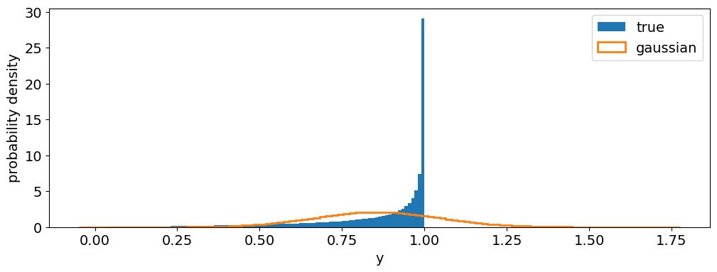
Figure 4 One million samples from a Beta distribution with $\alpha = 2$ and $\beta = \frac{1}{3}$ (blue histogram), and the corresponding gaussian approximation (orange curve). The idea behind a synthetic likelihood is to replace the blue probability density function with the orange one. This might look like a terrible idea, but in practice it tends to work!
This approximation cannot possibly be useful in inference... or can it? To find out, let's keep things simple and assume we know the true value of $\beta$. Our problem is therefore one-dimensional, so easy to solve numerically. We'll place a uniform prior on $\alpha$, so we can compute the posterior distribution by dividing the likelihood function by the evidence, which we compute by numerically integrating the likelihood over all values of $\alpha$.
import matplotlib.pyplot as plt

# True values
alpha_true = 2.0
beta_true = 0.33

# Array of alpha values to test
alpha_arr = np.linspace(1.5, 2.5, 1000)

# Let's simulate 50 different `y` datasets, each with k=1000 points
np.random.seed(0)
for k in range(50):

    # Draw our data: this is what we observe
    y = Beta.rvs(alpha_true, beta_true, size=1000)

    # Compute the log likelihood using the true likelihood function
    # Exponentiate it and divide by the evidence to get the posterior
    ll = np.array([log_likelihood(alpha, beta_true, y) for alpha in alpha_arr])
    ll -= np.nanmax(ll)
    pdf = np.exp(ll) / np.trapz(np.exp(ll))

    # Now do the same thing using the synthetic likelihood function
    ll_sl = np.array(
        [log_likelihood_synthetic(alpha, beta_true, y) for alpha in alpha_arr]
    )
    ll_sl -= np.nanmax(ll_sl)
    pdf_sl = np.exp(ll_sl) / np.trapz(np.exp(ll_sl))

    # Plot the two distributions
    plt.plot(alpha_arr, pdf, color="C0", alpha=0.25, lw=1)
    plt.plot(alpha_arr, pdf_sl, color="C1", alpha=0.25, lw=1)

plt.axvline(alpha_true, color="k", lw=1, ls="--", alpha=0.5)
If we run the code above, this is what we get:
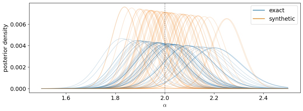
Figure 5 Posterior distributions for $\alpha$ given 50 different simulated $\mathbf{y}$ datasets, conditioned on the true value of $\beta$. Blue curves are the posteriors obtained using the true (correct) likelihood function. Orange curves are using the misspecified synthetic likelihood. The dashed vertical line shows the true value of $\alpha$.
We actually do really well! Both the exact and synthetic posteriors are centered (on average) on the true value, meaning the synthetic likelihood approach is in fact unbiased. The main difference, however, lies in the posterior variance: the orange PDFs (which use the synthetic likelihood)are taller and skinnier, even though they span about the same range in $\alpha$ over all datasets as the blue curves. This is a sign that something is wrong with our variance!
To test this, let's run this inference procedure on a lot more synthetic datasets: let's do 1,000 this time. In addition to computing the posterior, we can estimate the mean and variance by integrating to find the first two moments of the distribution. Here is the distribution of posterior means for $\alpha$$ over the 1,000 runs using the synthetic likelihood:
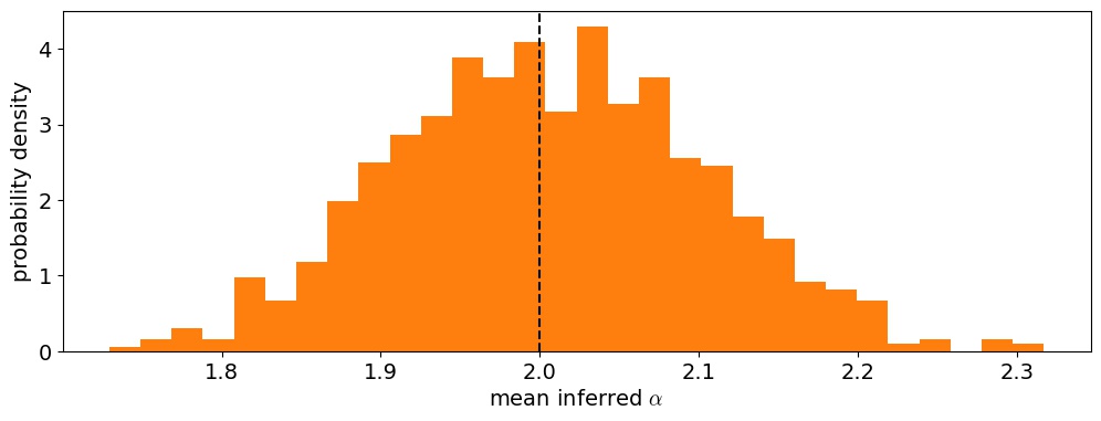
Figure 6 Distribution of posterior means for $\alpha$ under the synthetic likelihood model. The true value is indicated by the dashed vertical line.
As expected, the method is unbiased on average, which is excellent. Next, let's look at the distribution of normalized residuals. I compute these as
$$ \Delta_n = \frac{\mu_n - \alpha_\mathrm{true}}{\sigma_n} $$
where $\mu_n$ and $\sigma_n$ are the posterior mean and variance for the $n^\mathrm{th}$ simulation and $\alpha_\mathrm{true}$ is the true value of $\alpha$. If our posterior variances $\sigma_n^2$ are correct, then $\Delta$ should be distributed according to the standard normal:
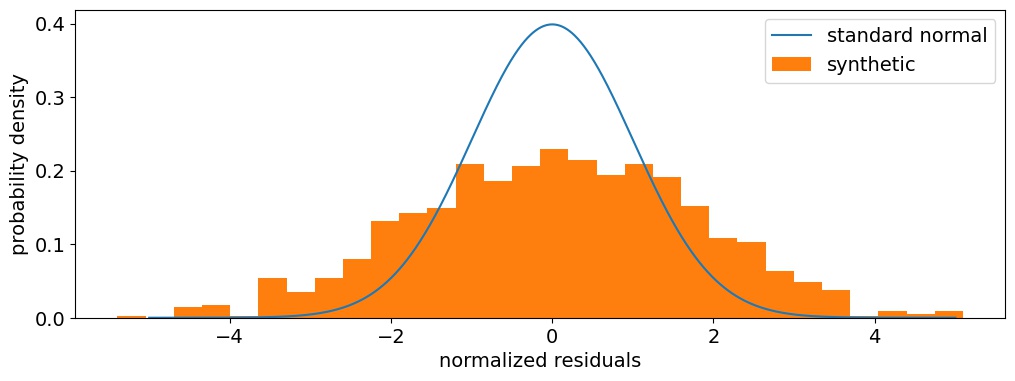
Figure 7 Distribution of normalized residuals, the difference between the posterior mean and the truth divided by the posterior standard deviation. The standard normal is overplotted in blue for reference.
Aha! The distribution of normalized residuals is wider than it should be, which means that the dispersion of posterior means is significantly wider than the individual posteriors. That confirms our suspicion from above that the synthetic likelihood method underestimates the posterior variance in this toy problem, by a factor of about 3 (alternatively, it underestimates the standard deviation by about 70 percent). So while the synthetic likelihood may be an unbiased estimator, it doesn't always provide a good estimate of the variance.
Closing Thoughts
In this post I discussed the idea behind a synthetic likelihood, which is pretty straightforward: if the true likelihood is difficult to calculate, we can instead try to find (or estimate) its first two moments and instead use the gaussian with the same mean and variance as our likelihood function. Surprisingly, this tends to yield unbiased posterior estimates, albeit with (slightly) wrong variance.
When I started writing this post I was hoping I could derive something a bit more rigorous about why the synthetic likelihood can't capture the variance correctly, but I haven't made any progress on that. In general, it doesn't seem to be too bad. In the much more complex inference problem I'm working on related to stellar surface mapping, I find just about the same results: the posterior means are unbiased, but the variances are underestimated by a small factor.
It's important to note that the magnitude of the discrepancy in the variance sensitively depends on the distribution you're trying to model. For different values of $\alpha$ and $\beta$ in the example above, I find that the synthetic likelihood underestimates the variance by different amounts, but rarely by more than in the example shown above. I suspect the issues with the variance occur when the distribution is very asymmetric or sharply peaked (as in this case), but I am very curious to hear other people's thoughts or ideas on this! As always, comments are welcome!
Finally, if you're interested in playing around with the toy model, you can find it here.
Rodrigo Luger
I'm a Flatiron Fellow at the CCA in New York City, working on a variety of things related to exoplanets, stars, and astronomical data analysis. I'm interested in systematics de-trending, the search for and characterization of potentially habitable exoplanets, and the mapping of stellar and exoplanetary surfaces from photometric and spectroscopic datasets. Outside the office I love to hike, bike, swim, craft lattes, faulty parallelism, and Oxford commas.