Interpretable GPs for stellar rotation (Part 2)
This is a continuation of the previous post, in which we implemented a very slow, inefficient, and numerically unstable Gaussian process for stellar light curves. In this post I'll discuss how to compute the GP kernel analytically and show how to use this GP to learn about star spot properties from stellar light curves.
Demo
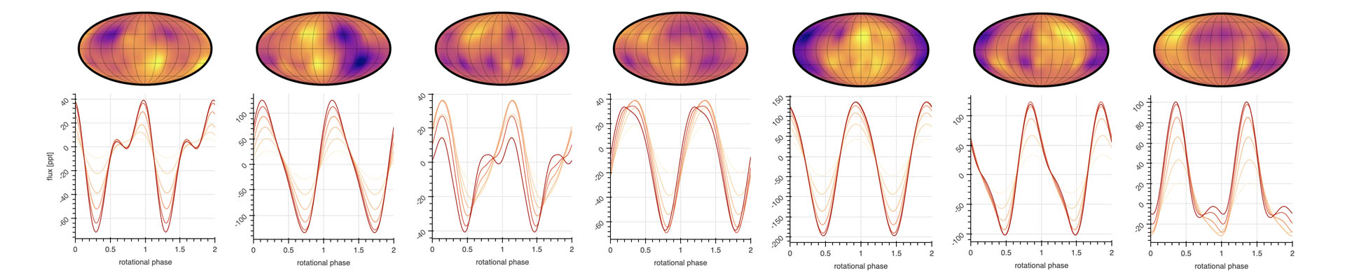
Before I discuss how any of this works, let's cut to the chase. Figure 1 below shows a demo of a starry process, a Gaussian process whose hyperparameters correspond to physical properties of the distribution of star spots on the stellar surface.
Figure 1 A video demo of a starry process. The kernel of the Gaussian process is a function of six hyperparameters that control the mean and standard deviation of the spot size, latitude, and contrast distributions (top panels). The bottom panels show random samples from the GP on the surface of the star (in a Mollweide projection) and in flux space. Line colors correspond to different stellar inclinations with respect to the line of sight. Because the kernel is an analytic function of the hyperparameters, drawing samples and computing marginal likelihoods with a starry process is extremely fast.
The kernel of the GP is a function of six parameters: the mean and standard deviation of the spot latitude distribution (in degrees; top left), the mean and standard deviation of the spot size distribution (also in degrees; top center), and the mean and standard deviation of the spot contrast (measured as a fraction of the photospheric intensity; top right). Below the distribution are five random samples from the GP, visualized on the surface of the star in an equal-area Mollweide projection. Below each are the corresponding light curves assuming different viewing inclinations ranging from 15° (yellow) to 90° (dark red). In the video, everything is computed in real time as the GP parameters are adjusted: because the starry process is analytic, it is extremely fast to evaluate.
The demo above is of course just a video. I'm hoping to turn it into a proper web app in the near future, but for the time being it has to be run locally. If you want to play around with it yourself, you can install the (very experimental) beta version as follows:
pip install "git+git://github.com/rodluger/starry_process.git@blog#egg=starry_process[app]"then, in the command line, type
starry-processto launch the Bokeh app.
What you can do with a starry process
Again, let's delay for the time being discussing how the GP works and briefly talk about what the GP can do. I mentioned in the previous post that an interpretable GP can be used within a hierarchical model to learn about ensemble statistics of many light curves. To recap, the idea behind this is that any individual light curve contains only a small fraction of the information about what the surface of the star looks like (because of all the degeneracies that come with projecting a two-dimensional surface down to a one-dimensional flux timeseries). However, these degeneracies are inclination-dependent, so different stars will have different degeneracies. The trick is to realize that if we collect light curves of many similar stars, we can learn more about the population than we can for any individual star. Here, similar is loosely defined: we simply want stars whose properties are drawn from the same parent distribution (individual stars may still look quite different!) To show how we can do this using a starry process, let's create a toy dataset:
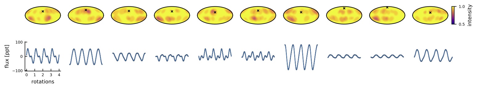
Figure 2 A synthetic dataset consisting of ten light curves of stars with similar star spot properties. The surface maps were generated by placing 20 discrete circular spots at latitudes and with sizes and contrasts drawn from fiducial Gaussian distributions. The light curves were then computed by expanding the surface in spherical harmonics to high degree (30) and using starry to compute fluxes. Each star was given a random inclination drawn from a \(\sin i\) prior; the \( \times \) on each map marks the sub-observer point. Finally, a small amount of noise was added to each light curve to simulate photon noise.
The figure above shows a dataset comprised of ten light curves of stars with statistically similar star spot properties. I generated it by choosing fiducial values for the mean and variance of the (Gaussian) distributions for the spot size, latitude, and contrast, then drawing 20 spots from these distributions for each star. The spots are circular and the contrast is uniform within each one (as we will see below, this is quite different from the prescription used to compute the GP; this is extremely important, since we don't want our proof that the GP works to be circular!) I then gave each star a random inclination, drawn from the expected \(\sin i\) prior for inclination angles, and computed the "observed" light curve using starry.
Now, we pretend we merely observe these light curves, and that we have absolutely no knowledge of the number of spots, the spot sizes, positions, and contrasts, or the inclination of any of the stars. (For simplicity, we'll assume we know the rotational period exactly, although this could easily be sampled over as well). The only thing we'll assume is that these stars are "similar": that is, there is some parent distribution from which all these stellar surfaces were drawn. In practice, this might mean the stars have the same spectral type, similar ages (or rotation periods), and similar metallicities. What we therefore do is to place uninformative priors on all of these quantities and use the sampler of our choice to explore their posteriors. Our likelihood function is the usual GP likelihood (see this equation), although this time our GP kernel is an explicit function of the parameters we care about. Figure 3 below shows the posterior distributions for some of the quantities of interest from a Variational Inference (VI) scheme:
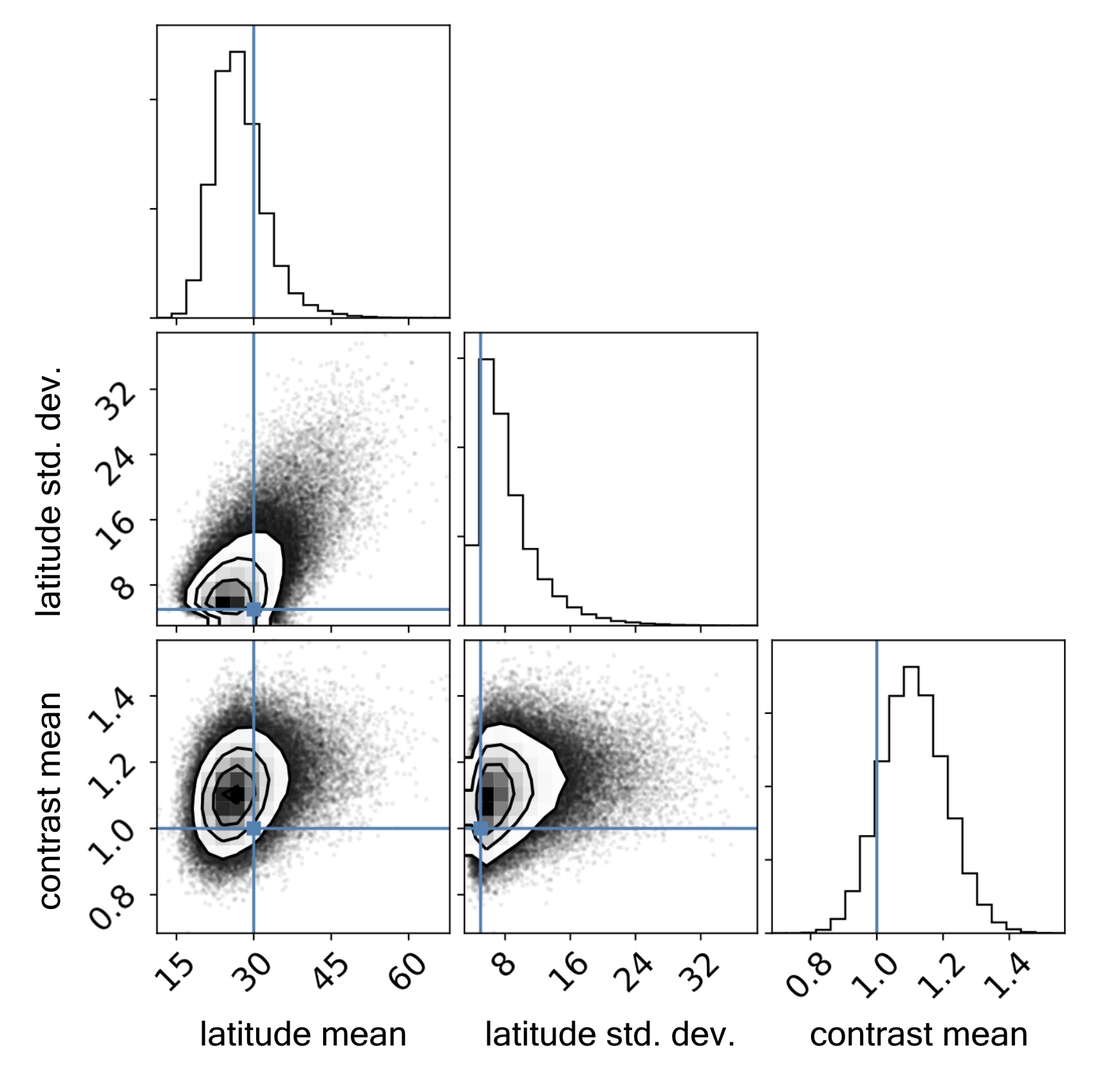
Figure 3 Joint posterior distributions for the hyperparameters governing the spot latitude and contrast distributions, inferred by jointly analyzing the ten light curves in Figure 2. Uniform priors were assumed for all hyperparameters of the GP. The inclinations of each star were also treated as latent variables (see Figure 4). The blue lines indicate the true values used to generate the synthetic dataset; note the excellent agreement with the inferred values.
As you can tell from the figure, we were able to accurately infer the mean latitude of the spots, the scatter (variance) in the latitude, and the typical contrast of the spots in our ensemble of ten stars. Below, Figure 4 shows the posterior distributions for the inclinations of each of the stars:
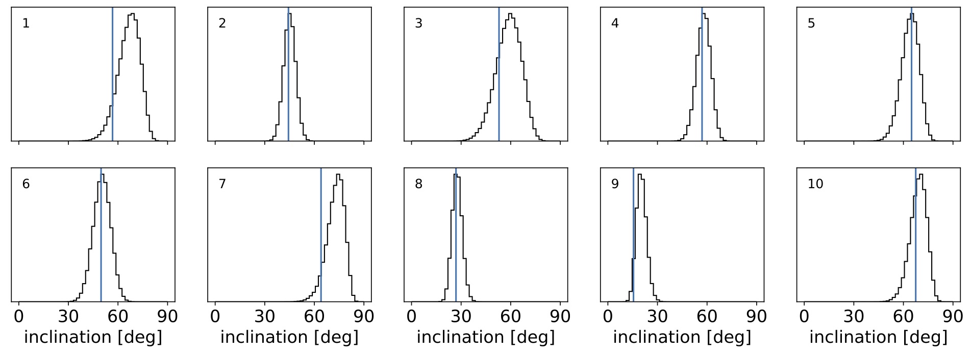
Figure 4 Posterior distributions for the inclinations of each of the ten stars in Figure 1. A \(\sin i\) prior was placed on each one. Stellar inclinations are notoriously difficult to infer from light curves given all the degeneracies in the mapping problem. However, ensemble analysis of similar stars allows one to infer these inclinations with fairly high precision and minimal bias.
Even though we assumed a completely uninformative inclination prior, we were able to infer the inclinations for all the stars in our sample with fairly good precision and minimal bias(!) This is something that is just not possible to do for a single star from its light curve, since the inclination is highly degenerate with the spot contrast, the number of spots, etc. This is the power of population-level analyses: the joint information content of lots of members allows us to learn not only population-level information (the typical latitude and contrast of the spots) but it also helps uncover information specific to individual members.
How it all works
In the previous post we talked about how to compute the mean and the covariance of the GP the brute force way: draw a huge number of samples from the desired distribution and then compute the empirical mean and covariance. That is super easy to do, but extremely inefficient (not to mention also very imprecise). What we need to do to make this GP scalable is to find closed form, analytic solutions for the GP mean and covariance. What follows is a (very rough) sketch of how to do this.
Let $\mathbf{f} = \left( f_0 \, f_1 \, \cdots \, f_K \right)^\top$ denote a vector of $K$ flux measurements at times $\left( t_0 \, t_1 \, \cdots \, t_K \right)^\top$; i.e., an observed light curve. Conditioned on certain physical properties of the star, $\pmb{\theta}$, we wish to compute the mean $\pmb{\mu}(\pmb{\theta})$ and covariance $\pmb{\Sigma}(\pmb{\theta})$ of $\mathbf{f}$, which together fully specify our Gaussian process. As with any random variable, the mean and covariance may be computed from the expectation value of $\mathbf{f}$ and $\mathbf{f}\,\mathbf{f}^\top$, respectively:
\begin{align} \label{eq:mean} \pmb{\mu}(\pmb{\theta}) & = \mathrm{E} \Big[ \mathbf{f} \, \Big| \, \pmb{\theta} \Big] \\ \label{eq:cov} \pmb{\Sigma}(\pmb{\theta}) & = \mathrm{E} \Big[ \mathbf{f} \, \mathbf{f}^\top \, \Big| \, \pmb{\theta} \Big] - \pmb{\mu}^2(\pmb{\theta}) \end{align}
where the squaring operation in Equation (\ref{eq:cov}) is shorthand for the outer product. In Luger et al. (2019) I showed that $\mathbf{f}$ may be computed from a linear operation on the vector of spherical harmonic coefficients describing the surface, $\mathbf{y}$:
\begin{align} \label{eq:fAy} \mathbf{f} = \mathbf{A} \, \mathbf{y} \quad, \end{align}
where $\mathbf{A}$ is the starry design matrix, which is implicitly a function of $\pmb{\theta}$ (as it depends on the stellar inclination and rotation period, for example). Given Equation (\ref{eq:fAy}), we may write the mean and covariance of our flux GP as
\begin{align} \pmb{\mu}(\pmb{\theta}) & = \mathbf{A}(\pmb{\theta}) \, \pmb{\mu}_{\mathbf{y}}(\pmb{\theta}) \\ \pmb{\Sigma}(\pmb{\theta}) & = \mathbf{A}(\pmb{\theta}) \, \pmb{\Sigma}_{\mathbf{y}} \, \mathbf{A}^\top(\pmb{\theta}) \quad, \end{align}
where
\begin{align} \label{eq:mean_y} \pmb{\mu}_{\mathbf{y}}(\pmb{\theta}) & = \mathrm{E} \Big[ \mathbf{y} \, \Big| \, \pmb{\theta} \Big] \\ \label{eq:cov_y} \pmb{\Sigma}_{\mathbf{y}}(\pmb{\theta}) & = \mathrm{E} \Big[ \mathbf{y} \, \mathbf{y}^\top \, \Big| \, \pmb{\theta} \Big] - \pmb{\mu}_{\mathbf{y}}^2(\pmb{\theta}) \end{align}
are the mean and covariance of the GP in the spherical harmonics basis. It's a lot of math, but under certain assumptions it's possible to compute the expectations in the expressions above analytically. These are given by the integrals
\begin{align} \label{eq:exp_y} \mathrm{E} \Big[ \mathbf{y} \, \Big| \, \pmb{\theta} \Big] & = \int \mathbf{y}(\mathbf{x} ) \, p(\mathbf{x} \, \big| \, \pmb{\theta})\mathrm{d}\mathbf{x} \\ \label{eq:exp_yy} \mathrm{E} \Big[ \mathbf{y} \, \mathbf{y}^\top \, \Big| \, \pmb{\theta} \Big] & = \int \mathbf{y}(\mathbf{x} ) \mathbf{y}^\top(\mathbf{x} ) \, p(\mathbf{x} \, \big| \, \pmb{\theta})\mathrm{d}\mathbf{x} \quad, \end{align}
where $\mathbf{x}$ is a random vector-valued variable corresponding to a particular distribution of features on the surface (i.e., the size and location of star spots) and $p(\mathbf{x} \, \big| \, \pmb{\theta})$ is its probability density function (PDF). As we are specifically interested in modeling the effect of star spots on stellar light curves, we let
\begin{align} \mathbf{x} = \left( \xi \,\, \lambda \,\, \phi \,\, \rho \right)^\top \end{align}
and
\begin{align} \label{eq:RRs} \mathbf{y}(\mathbf{x}) = \xi \, \mathbf{R}_{\hat{\mathbf{y}}}(\lambda) \, \mathbf{R}_{\hat{\mathbf{x}}}(\phi) \, \mathbf{s}(\rho) \quad, \end{align}
where $\xi$ is the contrast of a spot, $\lambda$ is its longitude, $\phi$ is its latitude, and $\rho$ is its radius. The vector function $\mathbf{s}(\rho)$ returns the spherical harmonic expansion of a negative unit brightness circular spot at $\lambda = \phi = 0$, $\mathbf{R}_{\hat{\mathbf{x}}}(\phi)$ is the Wigner matrix that rotates the expansion about $\hat{\mathbf{x}}$ such that the spot is centered at a latitude $\phi$, and $\mathbf{R}_{\hat{\mathbf{y}}}(\lambda)$ is the Wigner matrix that then rotates the expansion about $\hat{\mathbf{y}}$ such that the spot is centered at a longitude $\lambda$; these three functions are detailed in the sections below. Equation (\ref{eq:RRs}) thus provides a way of converting a random variable $\mathbf{x}$ describing the size, brightness, and position of a spot to the corresponding representation in terms of spherical harmonics. Note, importantly, that we are not interested in any specific value of $\mathbf{y}$; rather, we would like to know its expectation value under the probability distribution governing the different spot properties $\mathbf{x}$, i.e., $p(\mathbf{x} \, \big| \, \pmb{\theta})$. For simplicity, we assume that $p(\mathbf{x} \, \big| \, \pmb{\theta})$ is separable in each of the four spot properties:
\begin{align} p(\mathbf{x} \, \big| \, \pmb{\theta}) = p(\xi \, \big| \, \pmb{\theta}_{\xi}) \, p(\lambda \, \big| \, \pmb{\theta}_{\lambda}) \, p(\phi \, \big| \, \pmb{\theta}_{\phi})\, p(\rho \, \big| \, \pmb{\theta}_{\rho}) \quad, \end{align}
where
\begin{align} \pmb{\theta} = \left( \pmb{\theta}_{\xi} \, \, \pmb{\theta}_{\lambda} \, \, \pmb{\theta}_{\phi} \, \, \pmb{\theta}_{\rho} \right)^\top \end{align}
is the vector of hyperparameters of our GP. This allows us to rewrite the expectation integrals (\ref{eq:exp_y}) and (\ref{eq:exp_yy}) as
\begin{align} \label{eq:exp_y_sep} \mathrm{E} \Big[ \mathbf{y} \, \Big| \, \pmb{\theta} \Big] & = \mathbf{e_4}(\pmb{\theta}) \\[1em] \label{eq:exp_yy_sep} \mathrm{E} \Big[ \mathbf{y} \, \mathbf{y}^\top \, \Big| \, \pmb{\theta} \Big] & = \mathbf{E_4}(\pmb{\theta}) \end{align}
where we define the first moment integrals
\begin{align} \label{eq:e1} \mathbf{e_1}(\pmb{\theta}_\rho) & \equiv \int \mathbf{s}(\rho) \, p(\rho \, \big| \, \pmb{\theta}_{\rho}) \, \mathrm{d}\rho % \\[1em] % \label{eq:e2} \mathbf{e_2}(\pmb{\theta}_\phi, \mathbf{e_1}) & \equiv \int \mathbf{R}_{\hat{\mathbf{x}}}(\phi) \, \mathbf{e_1} \, p(\phi \, \big| \, \pmb{\theta}_{\phi}) \, \mathrm{d}\phi % \\[1em] % \label{eq:e3} \mathbf{e_3}(\pmb{\theta}_\lambda, \mathbf{e_2}) & \equiv \int \mathbf{R}_{\hat{\mathbf{y}}}(\lambda) \, \mathbf{e_2} \, p(\lambda \, \big| \, \pmb{\theta}_{\lambda}) \, \mathrm{d}\lambda \\[1em] \label{eq:e4} \mathbf{e_4}(\pmb{\theta}_\xi, \mathbf{e_3}) & \equiv \int \xi \, \mathbf{e_3} \, p(\xi \, \big| \, \pmb{\theta}_{\xi}) \, \mathrm{d}\xi % \end{align}
and the second moment integrals
\begin{align} \label{eq:E1} \mathbf{E_1}(\pmb{\theta}_\rho) & \equiv \int \mathbf{s}(\rho) \, \mathbf{s}^\top(\rho) \, p(\rho \, \big| \, \pmb{\theta}_{\rho}) \, \mathrm{d}\rho % \\[1em] % \label{eq:E2} \mathbf{E_2}(\pmb{\theta}_\phi, \mathbf{E_1}) & \equiv \int \mathbf{R}_{\hat{\mathbf{x}}}(\phi) \, \mathbf{E_1} \, \mathbf{E_1}^\top \, \mathbf{R}_{\hat{\mathbf{x}}}^\top(\phi) \, p(\phi \, \big| \, \pmb{\theta}_{\phi}) \mathrm{d}\phi % \\[1em] % \label{eq:E3} \mathbf{E_3}(\pmb{\theta}_\lambda, \mathbf{E_2}) & \equiv \int \mathbf{R}_{\hat{\mathbf{y}}}(\lambda) \, \mathbf{E_2} \, \mathbf{E_2}^\top \, \mathbf{R}_{\hat{\mathbf{y}}}^\top(\lambda) \, p(\lambda \, \big| \, \pmb{\theta}_{\lambda}) \mathrm{d}\phi \\[1em] % \label{eq:E4} \mathbf{E_4}(\pmb{\theta}_\xi, \mathbf{E_3}) & \equiv \int \xi^2 \, \mathbf{E_3} \, \mathbf{E_3}^\top \, p(\xi \, \big| \, \pmb{\theta}_\xi) \mathrm{d}\xi % \quad. \end{align}
The trick now is to find a functional form for the spherical harmonic expansion
of the spot, $\mathbf{s}(\rho)$, as well as for each of the probability
distributions
$p(\rho \, \big| \, \pmb{\theta}_{\rho})$,
$p(\phi \, \big| \, \pmb{\theta}_{\phi})$,
$p(\lambda \, \big| \, \pmb{\theta}_{\lambda})$,
and
$p(\xi \, \big| \, \pmb{\theta}_\xi)$,
such that the integrals above have closed-form expressions.
Note, importantly, that each integral is implicitly an integral of a vector
(in the case of the first moment integrals) or a matrix (in the case
of the second moment integrals), so we better
find analytic expressions for them (otherwise we'll spend a very long time
integrating each of the indices of each vector and matrix numerically).
I'm working on writing all this up into a paper, so I won't go any further into
the math in this blog post, other than to say that for a Lorentzian-like
star spot profile $\mathbf{s}(\rho)$, transformed Beta distributions for
$p(\rho \, \big| \, \pmb{\theta}_{\rho})$ and $p(\phi \, \big| \, \pmb{\theta}_{\phi})$,
and a log-Normal distribution for $p(\xi \, \big| \, \pmb{\theta}_\xi)$,
it is in fact possible to write down a closed-form solution to each of these
integrals. (Since we expect stars to be azimuthally symmetric on average,
$p(\lambda \, \big| \, \pmb{\theta}_{\lambda})$ is a uniform distribution over
$[0, 2\pi]$, so that's a relatively easy integral to take). If you're really
interested in the math behind all this, I'm working on the paper in
this github repository,
with the always up-to-date manuscript draft
here.
I'm also hoping to officially release the code soon. It's at the same github repository as the paper, and if you installed the app up top, you already have it on your computer. I'm still actively developing it, so there are likely still some bugs and the syntax might change a bit. There's also no documentation. But if you want to play around with it, here's an example of how to draw flux samples from a starry process:
from starry_process import StarryProcess
import matplotlib.pyplot as plt
import numpy as np

sp = StarryProcess(
    sa=0.3, sb=0.75, la=0.9, lb=0.7, ca=0.75, cb=0.0, period=1.0, inc=60.0
)
t = np.linspace(0, 3, 500)
flux = sp.sample(t, nsamples=10).eval()

for k in range(10):
    plt.plot(t, 1e3 * flux[k])

plt.xlabel("time [d]")
plt.ylabel("flux [ppt]")
plt.show()
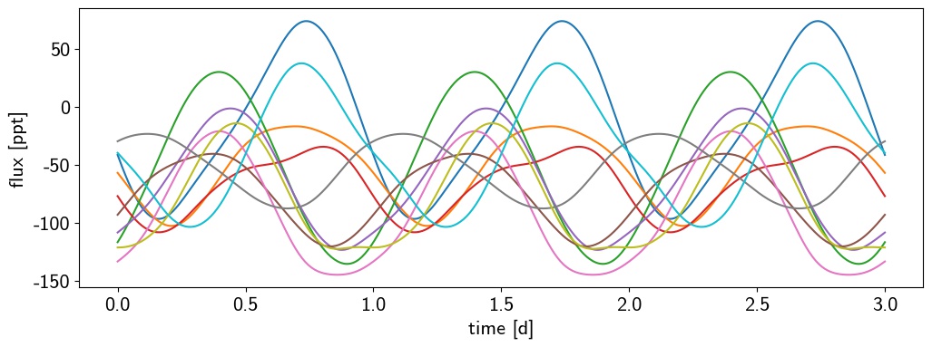
Figure 5 Flux samples from a starry process, generated from the code snippet above.
The parameters sa and sb are the normalized $\alpha$ and $\beta$ parameters of the Beta distribution controlling the spot size; the parameters la and lb are similar, but for the latitude distribution; ca and cb are the mean and variance of the log-Normal distribution for the spot contrast; and period and inc are the rotational period in days and inclination of the star in degrees. There is a one-to-one correspondence between parameters like sa and sb and the mean and variance of the spot size distribution (which are far more intuitive!), but I'll leave a more detailed discussion of this to the documentation (which I'm actively writing!)
Wrapping up
Hopefully I've convinced you that an interpretable Gaussian process is a useful development for stellar light curve analyses. This post only scratched the surface of how this GP works and what we can use it for, so I hope to write a lot more on this topic in coming posts. I'm also working on a paper describing the methodology and on making the code user-friendly and turning it into a pip-installable package. As always, feedback is extremely welcome!
Rodrigo Luger
I'm a Flatiron Fellow at the CCA in New York City, working on a variety of things related to exoplanets, stars, and astronomical data analysis. I'm interested in systematics de-trending, the search for and characterization of potentially habitable exoplanets, and the mapping of stellar and exoplanetary surfaces from photometric and spectroscopic datasets. Outside the office I love to hike, bike, swim, craft lattes, faulty parallelism, and Oxford commas.