Interpretable GPs for stellar rotation (Part 1)
As I discussed in my previous post, the information content of stellar light curves can be exceptionally tiny, owing to the large number of degeneracies when projecting from a two-dimensional space (the stellar surface) to a one-dimensional curve (the flux timeseries). Instead of trying to produce a definitive map of a stellar surface from a light curve, we can instead model the surface as a statistical process. In this post, I discuss ongoing work to develop a Gaussian process for stellar light curves whose hyperparameters are rooted in statistical properties of the stellar surface.
Ensemble Statistics
An important fact about the degeneracies in phase curves is that they are strong functions of the star's (or planet's) inclination. The surface modes we can constrain when the axis of rotation is at a right angle with respect to the line of sight (i.e., an inclination of 90°) are very different from those at inclinations of 60° or 45°. Since stellar inclinations are randomly distributed, we're able to learn slightly different things about the surfaces of different stars. This suggests that if we had enough stars, we could learn a lot more about the collective surface properties of that group of stars than we could for any individual star. This is the power of ensemble statistics: while individual light curves are only weakly informative, lots of light curves analyzed jointly can be extremely informative about statistics of the population.
But how do we harness this ensemble information? Thanks to Kepler and TESS, we now have access to hundreds of thousands of stellar light curves. We could imagine a scheme in which we select 1,000 light curves of "similar" TESS stars (say, 1,000 early M dwarfs with similar metallicity and rotation periods), and simultaneously fit for their surface maps. We do this simultaneously because we want to tie the individual maps together with priors shared by all stars: for example, the mean and variance of the spot size distribution, the mean and variance of the spot latitude distribution, etc. These priors are the hyperparameters of our model, the population-level statistics that we actually care about (see Figure 1).
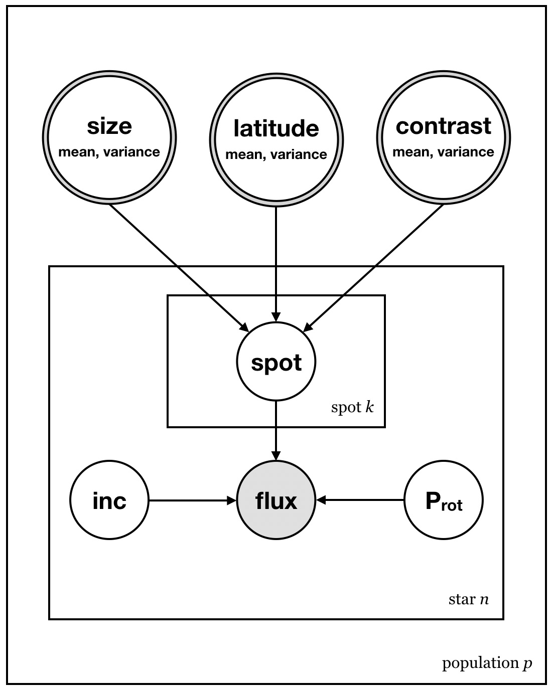
Figure 1 A probabilistic graphical model for stellar light curves. We model the surface of each star \(n\) in a population \(p\) of similar stars as the sum of \(k=1..K\) star spots. The properties of each spot (size, latitude, and contrast) are draws from a parent (hyper)distribution, whose means and variances are the global hyperparameters we wish to constrain.
Marginal Likelihood
In order for this scheme to work, we need to be able to compute the marginal likelihood function for each light curve: the probability that the observed data was drawn from a distribution with given hyperparameters. This is different from the probability of the data given a specific configuration of features on the surface of the star; rather, it is the probability integrated (or marginalized) over all possible surface brightness distributions consistent with the hyperparameters of the spot distribution. This is a tough integral no matter how you parametrize it. If we were to model stellar surfaces with discrete circular spots as in the figure above, we'd need to integrate over dozens — or maybe even hundreds — of free parameters for each star. That's a very tall order when your sample consists of 1,000 stars, even for modern MCMC and approximate inference methods.
Fortunately, there is one class of integrals that are very easy to compute: the integrals of Gaussian distributions. If the distribution from which the surface maps of the stars is drawn is a (multidimensional) Gaussian, we can analytically compute the required marginal likelihoods, turning an intractable high-dimensional integral into an easy sequence of operations in linear algebra. This is precisely the motivation behind Gaussian processes.
Nowadays, Gaussian processes are commonly used to model stellar variability, especially because of how efficient and simple to use they are. However, the choices made when fitting stellar light curves with GPs are often arbitrary: in particular, the kernel describing the covariance matrix is usually chosen to enforce a certain amount of smoothness in the model, but its functional form isn't inherently related to the star spots giving rise to the light curve variability. Nor are the kernel (hyper)parameters directly related to actual physical properties of the stars they are used to model (with the exception of the period, which is closely related to the rotation period of the star). An example of this is the ExpSineSquared kernel sometimes used for stellar light curves, which depends on a period parameter and a length scale parameter. The period may be interpreted as the rotation period of the star, but the meaning of the length scale is less obvious. It is related to the autocorrelation length of the light curve, which is in turn related to the autocorrelation length of features on the surface. But if we were given a light curve and tried to infer this length scale parameter (either by optimization or sampling), we wouldn't really know what to do with the value we obtain. For example, a short length scale could mean a surface covered in very small spots, or it could mean spots at a very low latitude, such that individual spots are only visible for a brief moment before returning to the backside of the star. Since our kernel wasn't specifically designed to capture stellar variability, we can't use it to learn anything useful about the spots on the surface.
Spherical Harmonics to the Rescue
Enter starry, the light curve modeling package I developed. starry models the surfaces of stars as linear combinations of spherical harmonics. One of the (many) cool things about spherical harmonics is their close relationship to Gaussian processes (sometimes called Gaussian Random Fields) on the sphere. If we consider expansions up to spherical harmonic degree \(l\), we can build a GP by constructing a covariance matrix of shape \( (l + 1)^2 \times (l + 1)^2 \). Cosmologists typically consider diagonal matrices, which define an isotropic Gaussian process whose power spectrum is related to the diagonal entries of this matrix. Drawing samples from this GP will yield vectors of spherical harmonic coefficients corresponding to different realizations of (say) the matter distribution in the Universe or (say) the surface brightness distribution of a stellar surface, conditioned on a given power spectrum. Alternatively, given an observation of one of these quantities (in our case, a stellar light curve), we can use the GP to compute the marginal likelihood of the dataset: the probability that this dataset was generated from the GP, integrating (marginalizing) over all possible configurations consistent with the parameters of the kernel.
In the cosmologists' case, an isotropic GP is often desirable, since (we believe) the Universe is isotropic on large scales. But in our case, we have reason to believe stellar surfaces are anisotropic, since the combined effects of rotation and magnetic fields tend to confine star spots to certain latitudes. On the sun, most spots form at mid-latitudes and migrate toward the equator over the course of a solar cycle. On other stars this may very well be different, but it is reasonable to assume that the azimuthal distribution of features may in general be different than the polar distribution: i.e., an anisotropic distribution.
In order to capture this anisotropy, we'll have to add off-diagonal terms to our covariance matrix. In an upcoming post I plan on discussing how to compute this covariance matrix in terms of the spot properties we are interested in, such as their size, latitudes, and contrasts. But for now, we can brute-force our way to the solution by computing this covariance matrix numerically.
Brute force GP
To start off, let's choose some fiducial values for our spot properties. Let's say we want to model a population of stars that have medium-sized spots (say of typical radius 10°) concentrated at mid-latitudes (say 30°) and with contrast of 10% on average. Let's further assume that each star in our population has 20 spots, each one drawn from some distribution with the means defined above and some small variance. We can use starry to generate these stars. Figure 2 shows five random draws from our spot distribution.
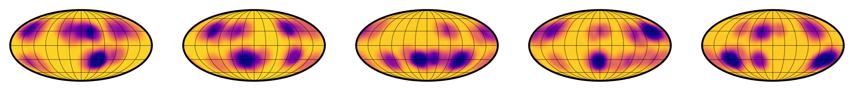
Figure 2 Five samples from the exact spot distribution. Each one corresponds to a spherical harmonic coefficient vector drawn from the spot size, position, and contrast distribution, visualized on a Mollweide projection on the stellar surface. This figure was generated from this python script.
Now, if we generate an infinite number of these maps, we could compute the mean and the covariance of the dataset. By definition, this will give us the mean and covariance of the multidimensional Gaussian distribution that best describes our input distribution: i.e., a Gaussian process model for our maps. While we can't really generate infinite maps, we can certainly generate a large number of them. Figure 3 shows the mean and covariance computed from 10,000 draws from our distribution.
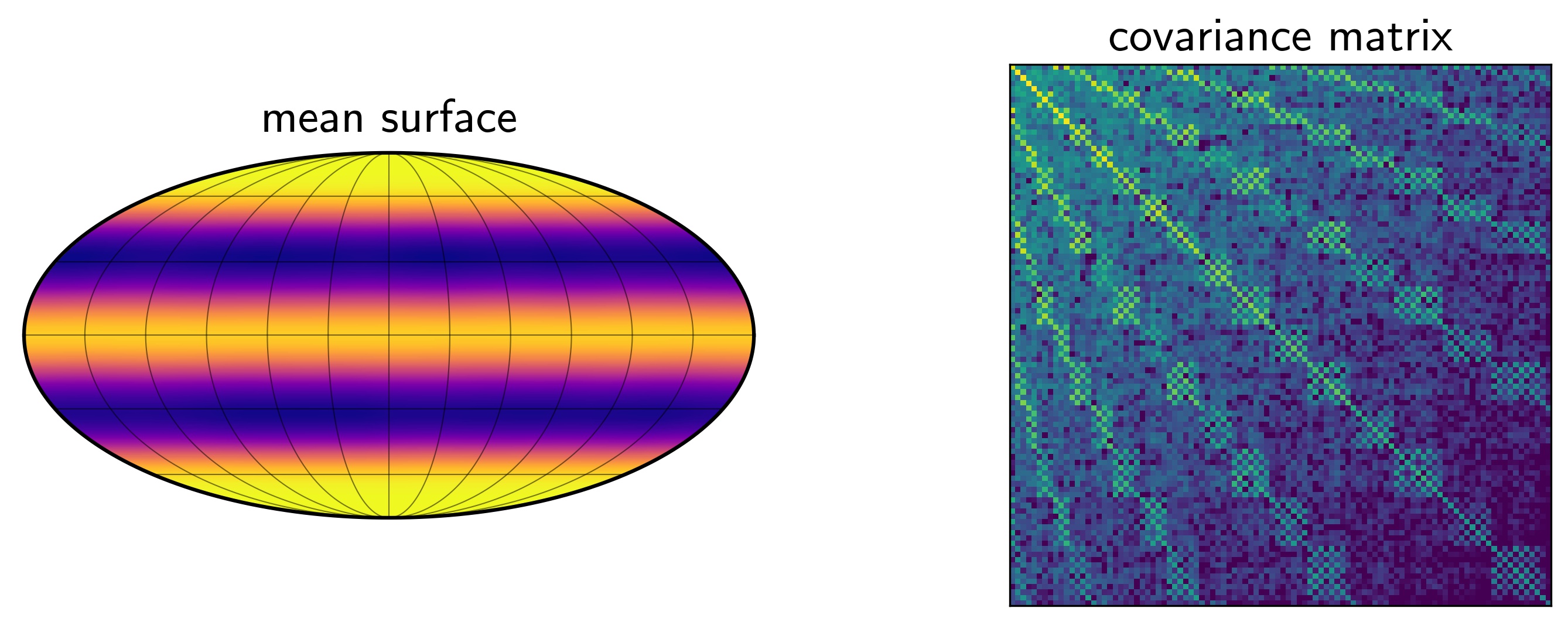
Figure 3 The empirical mean and covariance of our Gaussian process. Our GP is in the spherical harmonic basis, so the mean (left) corresponds to the mean spherical harmonic vector, which we're visualizing on a Mollweide projection on the stellar surface. The dark bands correspond to the average size and latitudinal extent of the star spots. The covariance is harder to visualize as a map, so we simply display the matrix itself as a colormap. Each entry in the matrix specifies the covariance between the spherical harmonic coefficients at indices given by the current row and column of the matrix. Note how complex the structure is, and in particular, the importance of the off-diagonal terms. This figure was generated from this python script.
Note that we can define our GP in whichever basis we'd like. But as we argued above, it's convenient to compute the GP in the spherical harmonic basis (as we will see in the next post, this actually allows us to compute things analytically!). The covariance matrix in the figure above therefore shows the correlation between spherical harmonic coefficients, and it's very complex — and distinctly non-diagonal. Note also that for every choice of the spot latitude, size, and contrast hyperparameters, we'll get different covariance matrices at this step.
Now that we have a GP, one of the things we can do is sample from it. Figure 4 shows five random draws from the GP:
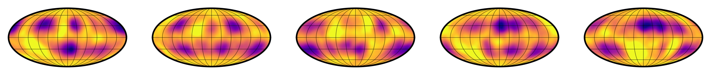
Figure 4 Five samples from our empirical Gaussian process. This figure was generated from this python script.
They kind of look like the samples from the exact distribution (Figure 2)! There are differences, of course: they are slightly noisier and sometimes contain bright spots in addition to dark spots. After all, the GP is only an approximation to the true distribution, but (as we will see in upcoming posts) it's a pretty good one.
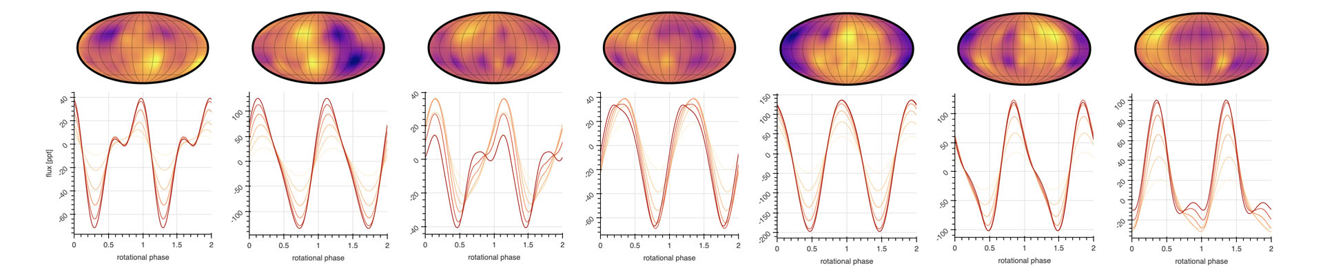
So far we've visualized our GP and its samples in the spherical harmonics basis, but we can easily rotate into the light curve basis. As I showed in this paper, the transformation from spherical harmonics to flux is linear, meaning we just have to take the product of the vector and a certain design matrix. Figure 5 shows the light curves corresponding to the map draws in the previous figure, visualized at different inclinations.
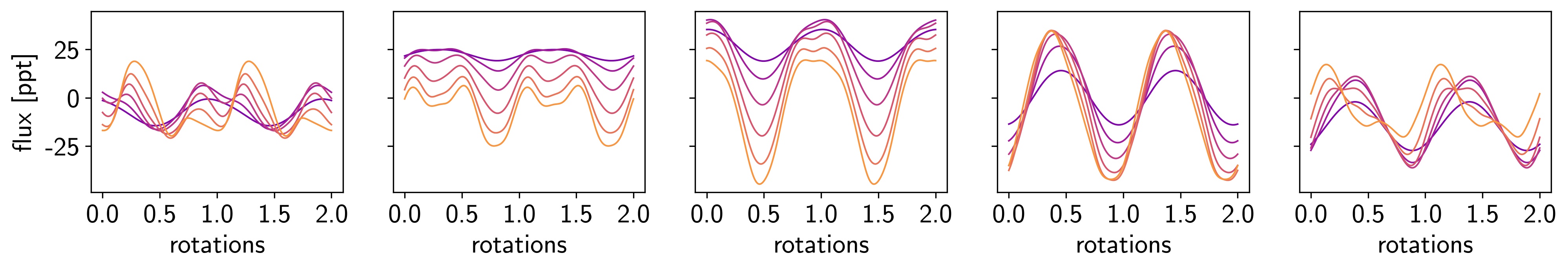
Figure 5 Five light curve samples from our empirical Gausssian process. These correspond to the light curves of the five maps shown in Figure 4, viewed at inclinations varying from 15° (dark purple) to 90° (light orange). This figure was generated from this python script.
Back to the Marginal Likelihood
Now, what we really would like to do is use this GP to compute likelihoods. Thanks to the amazing properties of Gaussians, that's also straightforward to do. If \( f \) is the flux (light curve) vector, \( C \) is the data covariance matrix (i.e., the uncertainties), and \( \mu \) and \( \Sigma \) are the GP mean and covariance (in flux space), respectively, the likelihood of the data given a set of GP hyperparameters \( \theta \) is

(see, e.g., this paper).
To do inference on a set of light curves — i.e., infer the star spot properties from the flux timeseries — we could use this as our likelihood function in, say, a Markov Chain Monte Carlo (MCMC) simulation, or as our (negative) loss function in an optimization scheme. However, this requires evaluating \( \mu(\theta) \) and \( \Sigma(\theta) \) for every combination of hyperparameters \(\theta\) we wish to explore. The covariance matrix in Figure 3 took about 20 seconds to compute, which is prohibitively long if you need to evaluate it tens to hundreds of thousands of times in an inference scheme. Plus, it's super noisy, as it's merely an empirical estimate of the true covariance.
In the next post, I'll discuss how to compute the covariance matrix (and the mean vector) analytically, in a fraction of a second and with minimal numerical error. Stay tuned!
Rodrigo Luger
I'm a Flatiron Fellow at the CCA in New York City, working on a variety of things related to exoplanets, stars, and astronomical data analysis. I'm interested in systematics de-trending, the search for and characterization of potentially habitable exoplanets, and the mapping of stellar and exoplanetary surfaces from photometric and spectroscopic datasets. Outside the office I love to hike, bike, swim, craft lattes, faulty parallelism, and Oxford commas.