Note

This tutorial was generated from a Jupyter notebook that can be downloaded here.

Eclipsing binary: pymc3 solution for the maps

In this notebook, we’re going to do MCMC to infer the surface maps of two stars in an eclipsing binary given the light curve of the system. We generated the data in this notebook. Note that here we assume we know everything else about the system (the orbital parameters, the limb darkening coefficients, etc.), so the only unknown parameters are the maps of the two stars, which are expressed in starry as vectors of spherical harmonic coefficients. In a future tutorial we’ll explore a more complex inference problem where we have uncertainties on all the parameters.

Let’s begin with some imports. Note that in order to do inference with pymc3, we need to enable lazy evaluation. That’s because pymc3 requires derivatives of the likelihood function, so we need to use the fancy theano computational graph to perform backpropagation on the starry model. All this means in practice is that we’ll have to call .eval() in some places to get numerical values out of the parameters.

import matplotlib.pyplot as plt
import numpy as np
import pymc3 as pm
import exoplanet as xo
import os
import starry
from corner import corner

np.random.seed(12)
starry.config.lazy = True
starry.config.quiet = True

Load the data

Let’s load the EB dataset:

data = np.load("eb.npz", allow_pickle=True)
A = data["A"].item()
B = data["B"].item()
t = data["t"]
flux = data["flux"]
sigma = data["sigma"]

Next, we instantiate the primary, secondary, and system objects. Recall that we assume we know the true values of all the orbital parameters and star properties, except for the two surface maps. Note that we are instantiating the starry objects within a pm.Model() context so that pymc3 can keep track of all the variables.

with pm.Model() as model:

    # Primary
    pri = starry.Primary(
        starry.Map(ydeg=A["ydeg"], udeg=A["udeg"], inc=A["inc"]),
        r=A["r"],
        m=A["m"],
        prot=A["prot"],
    )
    pri.map[1:] = A["u"]

    # Secondary
    sec = starry.Secondary(
        starry.Map(ydeg=B["ydeg"], udeg=B["udeg"], inc=B["inc"]),
        r=B["r"],
        m=B["m"],
        porb=B["porb"],
        prot=B["prot"],
        t0=B["t0"],
        inc=B["inc"],
    )
    sec.map[1:] = B["u"]

    # System
    sys = starry.System(pri, sec)

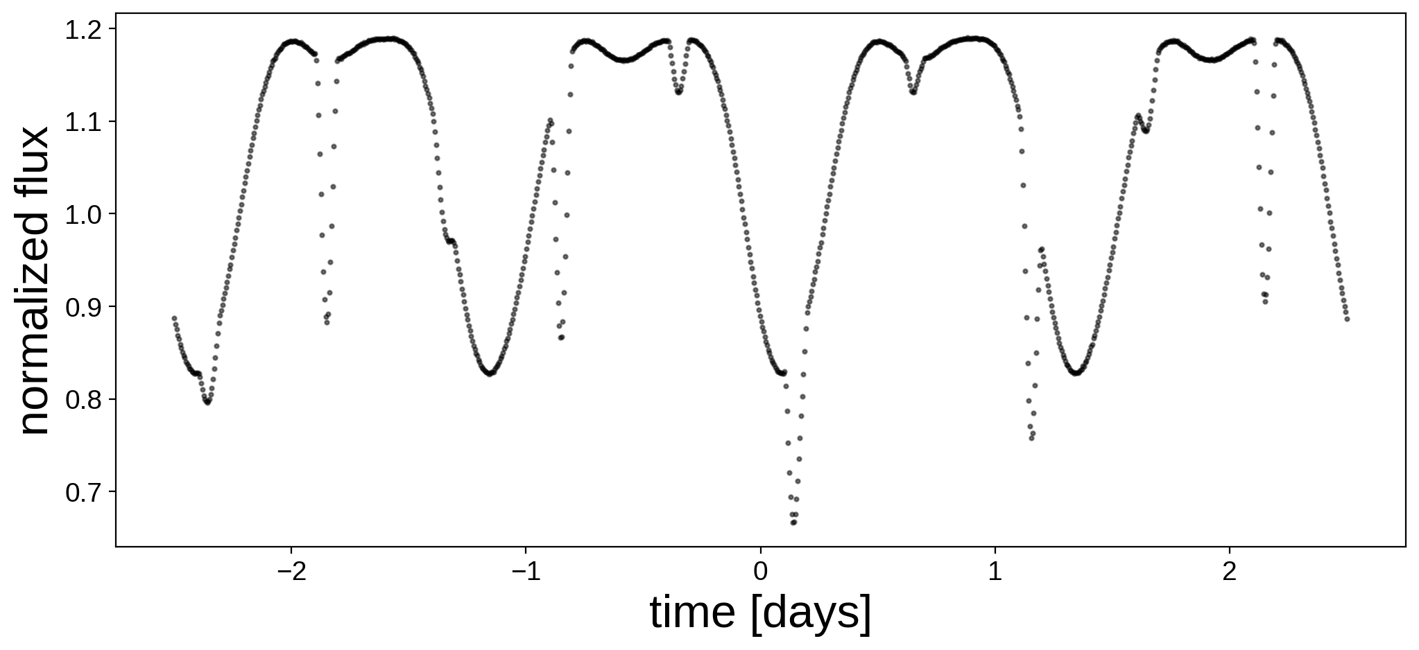
Here’s the light curve we’re going to do inference on:

fig, ax = plt.subplots(1, figsize=(12, 5))
ax.plot(t, flux, "k.", alpha=0.5, ms=4)
ax.set_xlabel("time [days]", fontsize=24)
ax.set_ylabel("normalized flux", fontsize=24);

Define the pymc3 model

Now we define the full pymc3 model. If you’ve never used pymc3 before, Dan Foreman-Mackey’s exoplanet package documentation has lots of nice tutorials on how to use pymc3 to do inference. The basic idea here is we define our variables by assigning priors to them; we use a pm.MvNormal for both the primary and secondary maps. This is a multi-variate normal (Gaussian) distribution, which happens to be a convenient prior to place on spherical harmonic coefficients because of its close relationship to the power spectrum of the map. In particular, if the Gaussian prior is zero-mean and its covariance is diagonal with constant entries for each degree \(l\) (as we assume below), this is equivalent to an isotropic prior whose power spectrum is given by those entries on the diagonal. Note that for simplicity we are assuming a flat power spectrum, meaning we place the same prior weight on all spatial scales. So the covariance of our Gaussian is as simple as it can be: it’s just \(\lambda I\), where \(\lambda = 10^{-2}\) is the prior variance of the spherical harmonic coefficients and \(I\) is the identity matrix. The scalar \(\lambda\) is essentially a regularization parameter: by making it small, we ensure that the spherical harmonic coefficients stay close to zero, which is usually what we want for physical maps.

You’ll note there’s also a call to pm.Deterministic, which just keeps track of variables for later (in this case, we’ll have access to the value of flux_model for every iteration of the chain once we’re done; this is useful for plotting). And finally, there’s a call to pm.Normal in which we specify our observed values, their standard deviation sd, and the mean vector mu, which is our starry flux model. This normal distribution is our chi-squared term: we’re telling pymc3 that our data is normally distributed about our model with some (observational) uncertainty.

with pm.Model() as model:

    # The amplitude of the primary
    pri.map.amp = pm.Normal("pri_amp", mu=1.0, sd=0.1)

    # The Ylm coefficients of the primary
    # with a zero-mean isotropic Gaussian prior
    ncoeff = pri.map.Ny - 1
    pri_mu = np.zeros(ncoeff)
    pri_cov = 1e-2 * np.eye(ncoeff)
    pri.map[1:, :] = pm.MvNormal("pri_y", pri_mu, pri_cov, shape=(ncoeff,))

    # The amplitude of the secondary
    sec.map.amp = pm.Normal("sec_amp", mu=0.1, sd=0.01)

    # The Ylm coefficients of the secondary
    # with a zero-mean isotropic Gaussian prior
    ncoeff = sec.map.Ny - 1
    sec_mu = np.zeros(ncoeff)
    sec_cov = 1e-2 * np.eye(ncoeff)
    sec.map[1:, :] = pm.MvNormal("sec_y", sec_mu, sec_cov, shape=(ncoeff,))

    # Compute the flux
    flux_model = sys.flux(t=t)

    # Track some values for plotting later
    pm.Deterministic("flux_model", flux_model)

    # Save our initial guess
    # See http://exoplanet.dfm.io/en/stable/user/api/#exoplanet.eval_in_model
    flux_model_guess = xo.eval_in_model(flux_model)

    # The likelihood function assuming known Gaussian uncertainty
    pm.Normal("obs", mu=flux_model, sd=sigma, observed=flux)

Now that we’ve specified the model, it’s a good idea to run a quick gradient descent to find the MAP (maximum a posteriori) solution. This will give us a decent starting point for the inference problem.

%%time
with model:
    map_soln = xo.optimize()

optimizing logp for variables: [sec_y, sec_amp, pri_y, pri_amp]
494it [00:02, 186.49it/s, logp=6.285776e+03]

CPU times: user 5.31 s, sys: 1.35 s, total: 6.65 s
Wall time: 43.2 s

message: Desired error not necessarily achieved due to precision loss.
logp: -33047316.911008343 -> 6285.775857961193

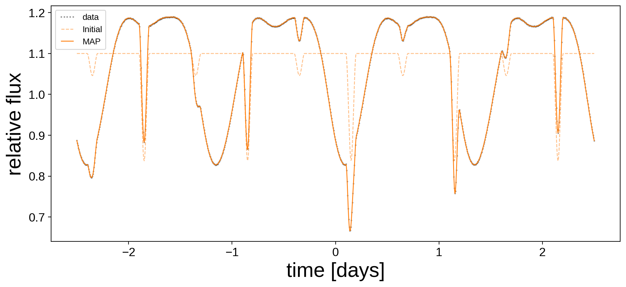
Note the dramatic increase in the value of the log posterior! Let’s plot the MAP model alongside the data and the initial guess (note that we’re doing quite well).

plt.figure(figsize=(12, 5))
plt.plot(t, flux, "k.", alpha=0.3, ms=2, label="data")
plt.plot(t, flux_model_guess, "C1--", lw=1, alpha=0.5, label="Initial")
plt.plot(
    t, xo.eval_in_model(flux_model, map_soln, model=model), "C1-", label="MAP", lw=1
)
plt.legend(fontsize=10, numpoints=5)
plt.xlabel("time [days]", fontsize=24)
plt.ylabel("relative flux", fontsize=24);

We can also plot the corresponding maps: note that we recover the spots really well!

map = starry.Map(ydeg=A["ydeg"])
map.inc = A["inc"]
map.amp = map_soln["pri_amp"]
map[1:, :] = map_soln["pri_y"]
map.show(theta=np.linspace(0, 360, 50))

map = starry.Map(ydeg=B["ydeg"])
map.inc = B["inc"]
map.amp = map_soln["sec_amp"]
map[1:, :] = map_soln["sec_y"]
map.show(theta=np.linspace(0, 360, 50))

MCMC sampling

We have an optimum solution, but we’re really interested in the posterior over surface maps (i.e., an understanding of the uncertainty of our solution). We’re therefore going to do MCMC sampling with pymc3. This is easy: within the model context, we just call pm.sample. The number of tuning and draw steps below are quite small since I wanted this notebook to run quickly; try increasing them by a factor of a few to get more faithful posteriors.

You can read about the get_dense_nuts_step convenience function (which really helps the sampling when degeneracies are present) here.

%%time
with model:
    trace = pm.sample(
        tune=500,
        draws=500,
        start=map_soln,
        chains=4,
        step=xo.get_dense_nuts_step(target_accept=0.9),
    )

Sequential sampling (4 chains in 1 job)
NUTS: [sec_y, sec_amp, pri_y, pri_amp]
Sampling chain 0, 40 divergences: 100%|██████████| 1000/1000 [03:40<00:00,  4.53it/s]
Sampling chain 1, 13 divergences: 100%|██████████| 1000/1000 [03:01<00:00,  5.51it/s]
Sampling chain 2, 5 divergences: 100%|██████████| 1000/1000 [03:26<00:00,  4.83it/s]
Sampling chain 3, 26 divergences: 100%|██████████| 1000/1000 [03:13<00:00,  5.17it/s]
There were 40 divergences after tuning. Increase `target_accept` or reparameterize.
The acceptance probability does not match the target. It is 0.7576036604307868, but should be close to 0.9. Try to increase the number of tuning steps.
There were 53 divergences after tuning. Increase `target_accept` or reparameterize.
The acceptance probability does not match the target. It is 0.8024727673914226, but should be close to 0.9. Try to increase the number of tuning steps.
There were 58 divergences after tuning. Increase `target_accept` or reparameterize.
The acceptance probability does not match the target. It is 0.8290602045619805, but should be close to 0.9. Try to increase the number of tuning steps.
There were 84 divergences after tuning. Increase `target_accept` or reparameterize.
The acceptance probability does not match the target. It is 0.8304876716026008, but should be close to 0.9. Try to increase the number of tuning steps.
The estimated number of effective samples is smaller than 200 for some parameters.

CPU times: user 15min 27s, sys: 1min 44s, total: 17min 12s
Wall time: 13min 41s

We can look at pm.summary to check if things converged. In particular, we’re looking for a large number of effective samples ess for all parameters and a value of r_hat that is very close to one.

varnames = ["pri_amp", "pri_y", "sec_amp", "sec_y"]
display(pm.summary(trace, var_names=varnames).head())
display(pm.summary(trace, var_names=varnames).tail())

	mean	sd	hpd_3%	hpd_97%	mcse_mean	mcse_sd	ess_mean	ess_sd	ess_bulk	ess_tail	r_hat
pri_amp	0.996	0.016	0.966	1.025	0.001	0.001	219.0	217.0	219.0	109.0	1.02
pri_y[0]	-0.019	0.034	-0.086	0.042	0.002	0.001	296.0	296.0	321.0	131.0	1.01
pri_y[1]	-0.112	0.003	-0.118	-0.106	0.000	0.000	468.0	468.0	480.0	265.0	1.01
pri_y[2]	0.065	0.003	0.060	0.071	0.000	0.000	875.0	875.0	898.0	401.0	1.01
pri_y[3]	0.003	0.024	-0.042	0.047	0.001	0.001	882.0	683.0	895.0	449.0	1.00

	mean	sd	hpd_3%	hpd_97%	mcse_mean	mcse_sd	ess_mean	ess_sd	ess_bulk	ess_tail	r_hat
sec_y[30]	0.009	0.023	-0.032	0.051	0.001	0.000	2008.0	1265.0	2007.0	1820.0	1.00
sec_y[31]	0.033	0.051	-0.072	0.117	0.002	0.001	634.0	634.0	640.0	513.0	1.01
sec_y[32]	-0.011	0.041	-0.095	0.061	0.001	0.001	1921.0	1160.0	1905.0	1408.0	1.00
sec_y[33]	0.045	0.049	-0.041	0.140	0.001	0.001	2272.0	1501.0	2283.0	1647.0	1.00
sec_y[34]	-0.047	0.063	-0.170	0.061	0.002	0.001	1741.0	1405.0	1735.0	1090.0	1.00

The number of effective samples for some of the parameters is quite small, so in practice we should run this chain for longer (an exercise for the reader!) But let’s carry on for now, keeping in mind that our posteriors will be quite noisy.

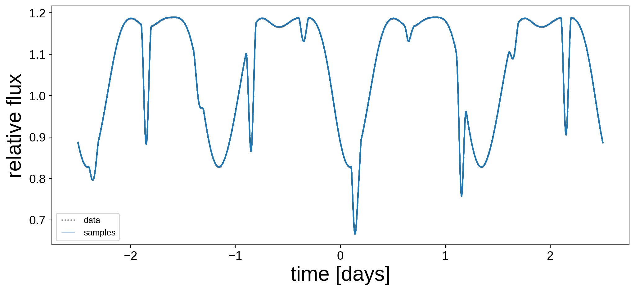
Let’s plot the model for 24 random samples from the chain. Note that the lines are so close together that they’re indistinguishable!

plt.figure(figsize=(12, 5))
plt.plot(t, flux, "k.", alpha=0.3, ms=2, label="data")
label = "samples"
for i in np.random.choice(range(len(trace["flux_model"])), 24):
    plt.plot(t, trace["flux_model"][i], "C0-", alpha=0.3, label=label)
    label = None
plt.legend(fontsize=10, numpoints=5)
plt.xlabel("time [days]", fontsize=24)
plt.ylabel("relative flux", fontsize=24);

Let’s compare the mean map and a random sample to the true map for each star:

# Random sample
np.random.seed(0)
i = np.random.randint(len(trace["pri_y"]))

map = starry.Map(ydeg=A["ydeg"])
map[1:, :] = np.mean(trace["pri_y"], axis=0)
map.amp = np.mean(trace["pri_amp"])
pri_mu = map.render(projection="rect").eval()
map[1:, :] = trace["pri_y"][i]
map.amp = trace["pri_amp"][i]
pri_draw = map.render(projection="rect").eval()
map[1:, :] = A["y"]
map.amp = A["amp"]
pri_true = map.render(projection="rect").eval()

map = starry.Map(ydeg=B["ydeg"])
map[1:, :] = np.mean(trace["sec_y"], axis=0)
map.amp = np.mean(trace["sec_amp"])
sec_mu = map.render(projection="rect").eval()
map[1:, :] = trace["sec_y"][i]
map.amp = trace["sec_amp"][i]
sec_draw = map.render(projection="rect").eval()
map[1:, :] = B["y"]
map.amp = B["amp"]
sec_true = map.render(projection="rect").eval()

fig, ax = plt.subplots(3, 2, figsize=(8, 7))
ax[0, 0].imshow(
    pri_true,
    origin="lower",
    extent=(-180, 180, -90, 90),
    cmap="plasma",
    vmin=0,
    vmax=0.4,
)
ax[1, 0].imshow(
    pri_mu,
    origin="lower",
    extent=(-180, 180, -90, 90),
    cmap="plasma",
    vmin=0,
    vmax=0.4,
)
ax[2, 0].imshow(
    pri_draw,
    origin="lower",
    extent=(-180, 180, -90, 90),
    cmap="plasma",
    vmin=0,
    vmax=0.4,
)
ax[0, 1].imshow(
    sec_true,
    origin="lower",
    extent=(-180, 180, -90, 90),
    cmap="plasma",
    vmin=0,
    vmax=0.04,
)
ax[1, 1].imshow(
    sec_mu,
    origin="lower",
    extent=(-180, 180, -90, 90),
    cmap="plasma",
    vmin=0,
    vmax=0.04,
)
ax[2, 1].imshow(
    sec_draw,
    origin="lower",
    extent=(-180, 180, -90, 90),
    cmap="plasma",
    vmin=0,
    vmax=0.04,
)
ax[0, 0].set_title("primary")
ax[0, 1].set_title("secondary")
ax[0, 0].set_ylabel("true", rotation=0, labelpad=20)
ax[1, 0].set_ylabel("mean", rotation=0, labelpad=20)
ax[2, 0].set_ylabel("draw", rotation=0, labelpad=20);

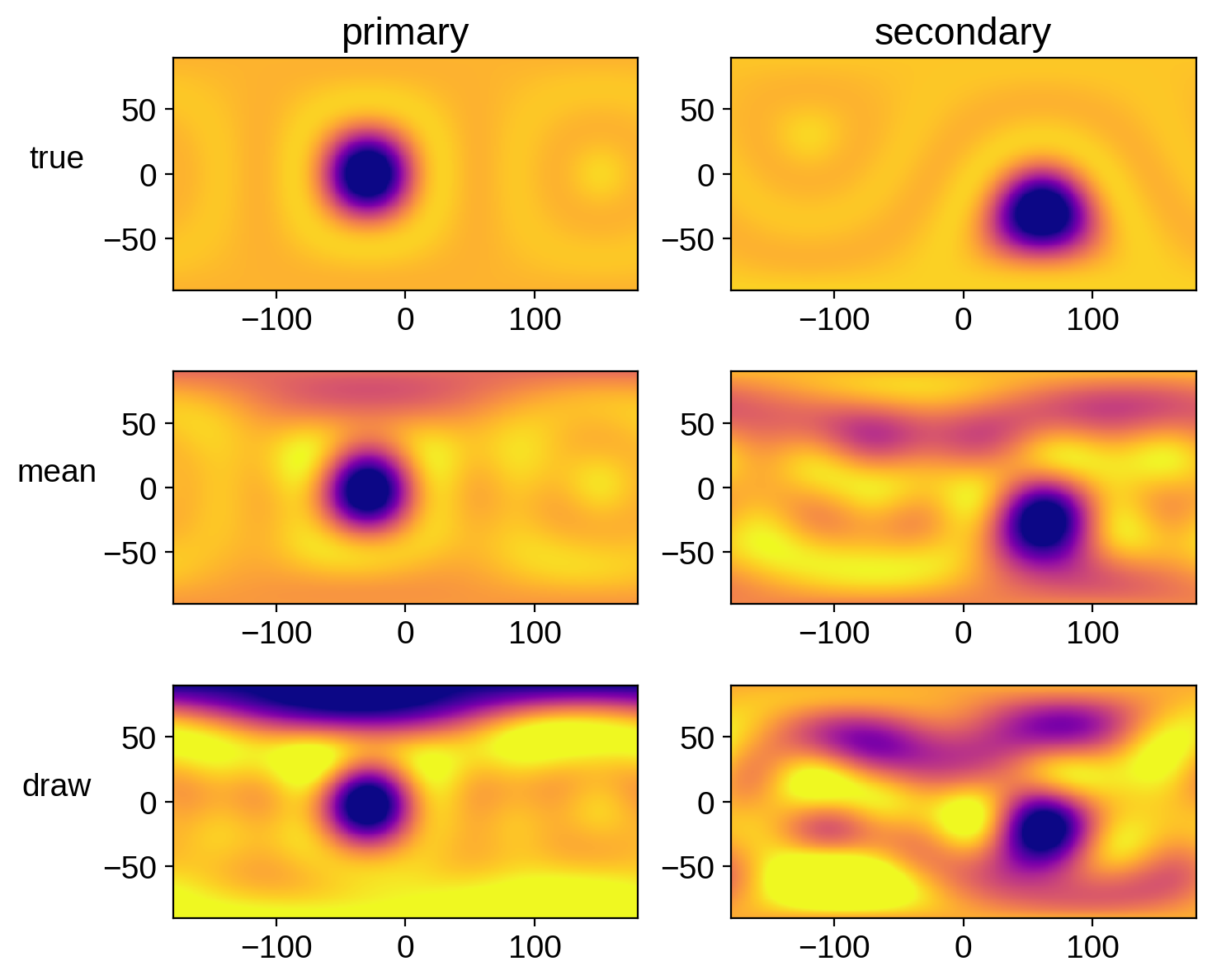
Looks pretty good! There are obvious artifacts (there are tons of degeneracies in this problem), but we’ve definitely recovered the spots, with some uncertainty. Recall that our chains weren’t well converged! Run this notebook for longer to get more faithful posteriors.

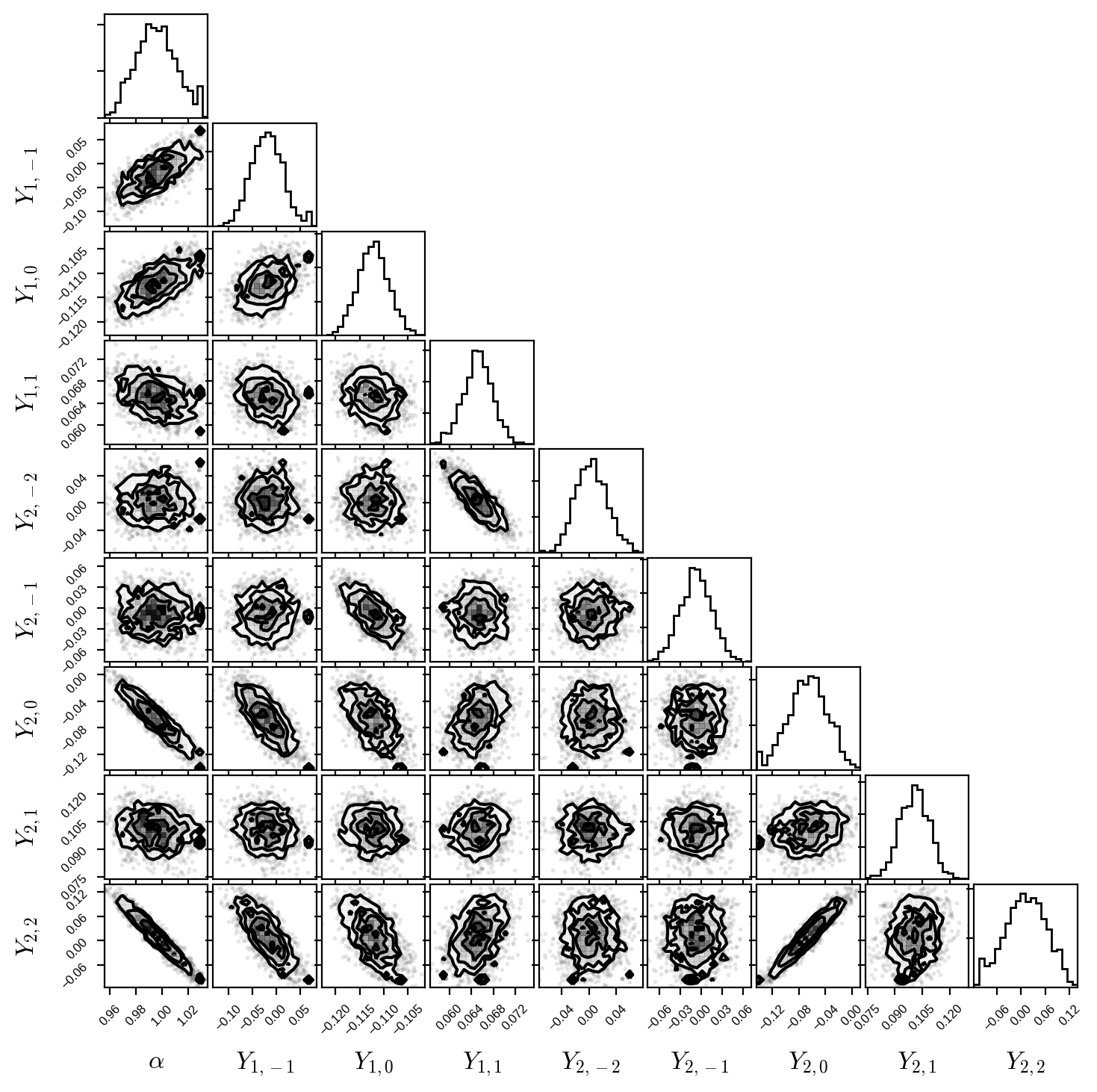
Finally, here’s a corner plot for the first several coefficients of the primary map. You can see that all the posteriors are nice and Gaussian, with some fairly strong correlations (the degeneracies I mentioned above):

fig, ax = plt.subplots(9, 9, figsize=(7, 7))
labels = [r"$\alpha$"] + [
    r"$Y_{%d,%d}$" % (l, m)
    for l in range(1, pri.map.ydeg + 1)
    for m in range(-l, l + 1)
]
samps = np.hstack((trace["pri_amp"].reshape(-1, 1), trace["pri_y"][:, :8]))
corner(samps, fig=fig, labels=labels)
for axis in ax.flatten():
    axis.xaxis.set_tick_params(labelsize=6)
    axis.yaxis.set_tick_params(labelsize=6)
    axis.xaxis.label.set_size(12)
    axis.yaxis.label.set_size(12)
    axis.xaxis.set_label_coords(0.5, -0.6)
    axis.yaxis.set_label_coords(-0.6, 0.5)

That’s it! While sampling with pymc3 is fairly fast, the problem of inferring a surface map when all other parameters are known is a linear problem, which means it actually has an analytic solution! In the following notebook, we show how to take advantage of this within starry to do extremely fast inference.