Note

This tutorial was generated from a Jupyter notebook that can be downloaded here.

Eclipsing binary: Solving for everything the slow way

In this notebook, we’re continuing our tutorial on how to do inference. In this notebook we showed how to use pymc3 to get posteriors over map coefficients of an eclipsing binary light curve, and in this notebook we did the same thing using the analytic linear formalism of starry.

Here, we are going to solve for everything: the map coefficients and all the orbital parameters of the system. Note that this is an expensive problem to solve (typically several hours on a laptop) since we need to sample in la very high dimensional and somewhat complex space. In this notebook, we use pymc3 to sample in all the parameters, including the map coefficients. This is therefore the slow way of doing this. As we will see in the next notebook, we can take advantage of the best of both worlds: sample the non-linear orbital parameters while analytically marginalizing over the map coefficients. Here, however, we’ll solve the full problem using pymc3 for comparison later.

Note that since we’re using pymc3, we need to enable lazy evaluation mode in starry.

import matplotlib
import matplotlib.pyplot as plt
import numpy as np
import pymc3 as pm
import exoplanet as xo
import os
import starry
from corner import corner
import theano.tensor as tt
from tqdm.notebook import tqdm

np.random.seed(12)
starry.config.lazy = True
starry.config.quiet = True

Load the data

Let’s load the EB dataset:

data = np.load("eb.npz", allow_pickle=True)
A = data["A"].item()
B = data["B"].item()
t = data["t"]
flux = data["flux"]
sigma = data["sigma"]

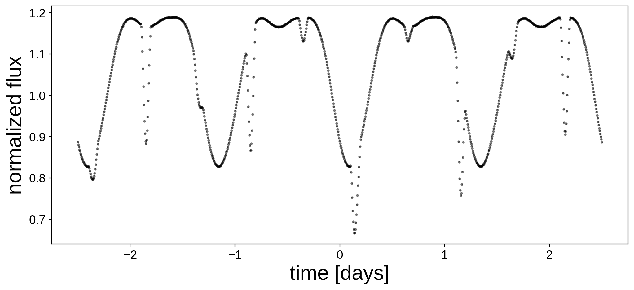
Here’s the light curve we’re going to do inference on:

fig, ax = plt.subplots(1, figsize=(12, 5))
ax.plot(t, flux, "k.", alpha=0.5, ms=4)
ax.set_xlabel("time [days]", fontsize=24)
ax.set_ylabel("normalized flux", fontsize=24);

We now instantiate the primary, secondary, and system objects within a pm.Model() context. Here are the priors we are going to assume for the parameters of the primary:

Parameter	True Value	Assumed Value / Prior	Units
$\mathrm{amp}$	$1.0$	$\mathcal{N}(1.0,0.1^2)$	$-$
$r$	$1.0$	$\mathcal{N}(0.95,0.1^2)$	$R_\odot$
$m$	$1.0$	$\mathcal{N}(1.05,0.1^2)$	$M_\odot$
$P_\mathrm{rot}$	$1.25$	$\mathcal{N}(1.25,0.01^2)$	$\mathrm{days}$
$i$	$80.0$	$\mathcal{N}(80.0,5.0^2)$	$\mathrm{deg}$
$u_1$	$0.40$	$0.40$	$-$
$u_2$	$0.25$	$0.25$	$-$

And here are the priors we are going to assume for the secondary:

Parameter	True Value	Assumed Value / Prior	Units
$\mathrm{amp}$	$0.1$	$\mathcal{N}(0.1,0.01^2)$	$-$
$r$	$0.7$	$\mathcal{N}(0.75,0.1^2)$	$R_\odot$
$m$	$0.7$	$\mathcal{N}(0.70,0.1^2)$	$M_\odot$
$P_\mathrm{rot}$	$0.625$	$\mathcal{N}(0.625,0.01^2)$	$\mathrm{days}$
$P_\mathrm{orb}$	$1.0$	$\mathcal{N}(1.01,0.01^2)$	$\mathrm{days}$
$t_0$	$0.15$	$\mathcal{N}(0.15,0.001^2)$	$\mathrm{days}$
$i$	$80.0$	$\mathcal{N}(80.0,5.0^2)$	$\mathrm{deg}$
$e$	$0.0$	$0.0$	$-$
$\Omega$	$0.0$	$0.0$	$\mathrm{deg}$
$u_1$	$0.20$	$0.20$	$-$
$u_2$	$0.05$	$0.05$	$-$

Above, $\mathcal{N}$ denotes a 1-d normal prior with a given mean and variance. Note that for simplicity we are fixing the limb darkening coefficients at their true value.

As in the previous notebooks, we’ll assume a gaussian priors for both sets of spherical harmonic coefficients.

with pm.Model() as model:

    # Some of the gaussians have significant support at < 0
    # Let's force them to be positive (required for quantites
    # such as radius, mass, etc.)
    # NOTE: When using `pm.Bound`, it is *very important* to
    # explicitly define a `testval` -- otherwise this defaults
    # to unity. Since the `testval` is used to initialize the
    # optimization step, it's very important we start at
    # reasonable values, otherwise things will never converge!
    PositiveNormal = pm.Bound(pm.Normal, lower=0.0)

    # Primary
    A_inc = pm.Normal("A_inc", mu=80, sd=5, testval=80)
    A_amp = pm.Normal("A_amp", mu=1.0, sd=0.1, testval=1.0)
    A_r = PositiveNormal("A_r", mu=0.95, sd=0.1, testval=0.95)
    A_m = PositiveNormal("A_m", mu=1.05, sd=0.1, testval=1.05)
    A_prot = PositiveNormal("A_prot", mu=1.25, sd=0.01, testval=1.25)
    pri = starry.Primary(
        starry.Map(ydeg=A["ydeg"], udeg=A["udeg"], inc=A_inc, amp=A_amp),
        r=A_r,
        m=A_m,
        prot=A_prot,
    )
    pri.map[1] = A["u"][0]
    pri.map[2] = A["u"][1]

    # The Ylm coefficients of the primary
    # with a zero-mean isotropic Gaussian prior
    ncoeff = pri.map.Ny - 1
    pri_mu = np.zeros(ncoeff)
    pri_cov = 1e-2 * np.eye(ncoeff)
    pri.map[1:, :] = pm.MvNormal("pri_y", pri_mu, pri_cov, shape=(ncoeff,))

    # Secondary
    B_inc = pm.Normal("B_inc", mu=80, sd=5, testval=80)
    B_amp = pm.Normal("B_amp", mu=0.1, sd=0.01, testval=0.1)
    B_r = PositiveNormal("B_r", mu=0.75, sd=0.1, testval=0.75)
    B_m = PositiveNormal("B_m", mu=0.70, sd=0.1, testval=0.70)
    B_prot = PositiveNormal("B_prot", mu=0.625, sd=0.01, testval=0.625)
    B_porb = PositiveNormal("B_porb", mu=1.01, sd=0.01, testval=1.01)
    B_t0 = pm.Normal("B_t0", mu=0.15, sd=0.001, testval=0.15)
    sec = starry.Secondary(
        starry.Map(ydeg=B["ydeg"], udeg=B["udeg"], inc=B_inc, amp=B_amp),
        r=B_r,
        m=B_m,
        porb=B_porb,
        prot=B_prot,
        t0=B_t0,
        inc=B_inc,
    )
    sec.map[1] = B["u"][0]
    sec.map[2] = B["u"][1]

    # The Ylm coefficients of the secondary
    # with a zero-mean isotropic Gaussian prior
    ncoeff = sec.map.Ny - 1
    sec_mu = np.zeros(ncoeff)
    sec_cov = 1e-2 * np.eye(ncoeff)
    sec.map[1:, :] = pm.MvNormal("sec_y", sec_mu, sec_cov, shape=(ncoeff,))

    # System
    sys = starry.System(pri, sec)

    # Compute the flux
    flux_model = sys.flux(t=t)

    # Track some values for plotting later
    pm.Deterministic("flux_model", flux_model)

    # Save our initial guess
    flux_model_guess = xo.eval_in_model(flux_model)

    # The likelihood function assuming known Gaussian uncertainty
    pm.Normal("obs", mu=flux_model, sd=sigma, observed=flux)

Now that we’ve specified the model, we run gradient descent to find the best fit solution. This will give us a decent starting point for the inference problem.

NOTE: Because we have so many parameters, it’s a bad idea to try to optimize everything at once. We’ll therefore iterate back and forth a few times between optimizing the surface maps and optimizing the orbital parameters.

with model:
    map_soln = xo.optimize(
        vars=[A_inc, A_r, A_m, A_prot, B_inc, B_r, B_m, B_prot, B_porb, B_t0],
        start=model.test_point,
    )

optimizing logp for variables: [B_t0, B_porb, B_prot, B_m, B_r, B_inc, A_prot, A_m, A_r, A_inc]
146it [00:03, 37.08it/s, logp=-3.290297e+07]
message: Desired error not necessarily achieved due to precision loss.
logp: -34272685.68890266 -> -32902974.30527578

with model:
    map_soln = xo.optimize(
        vars=[A_amp, pri.map[1:, :], B_amp, sec.map[1:, :]], start=map_soln
    )

optimizing logp for variables: [sec_y, B_amp, pri_y, A_amp]
837it [00:05, 158.47it/s, logp=3.807872e+03]
message: Desired error not necessarily achieved due to precision loss.
logp: -32902974.30527578 -> 3807.8722091388668

with model:
    map_soln = xo.optimize(
        vars=[A_inc, A_r, A_m, A_prot, B_inc, B_r, B_m, B_prot, B_porb, B_t0],
        start=map_soln,
    )

optimizing logp for variables: [B_t0, B_porb, B_prot, B_m, B_r, B_inc, A_prot, A_m, A_r, A_inc]
109it [00:02, 43.42it/s, logp=4.217677e+03]
message: Desired error not necessarily achieved due to precision loss.
logp: 3807.8722091388668 -> 4217.677137360188

with model:
    map_soln = xo.optimize(start=map_soln)

optimizing logp for variables: [sec_y, B_t0, B_porb, B_prot, B_m, B_r, B_amp, B_inc, pri_y, A_prot, A_m, A_r, A_amp, A_inc]
1719it [00:27, 62.65it/s, logp=6.307507e+03]
message: Desired error not necessarily achieved due to precision loss.
logp: 4217.677137360188 -> 6307.506745198042

Let’s see how we did:

plt.figure(figsize=(12, 5))
plt.plot(t, flux, "k.", alpha=0.3, ms=2, label="data")
plt.plot(t, flux_model_guess, "C1--", lw=1, alpha=0.5, label="Initial")
plt.plot(
    t, xo.eval_in_model(flux_model, map_soln, model=model), "C1-", label="MAP", lw=1
)
plt.legend(fontsize=10, numpoints=5)
plt.xlabel("time [days]", fontsize=24)
plt.ylabel("relative flux", fontsize=24);

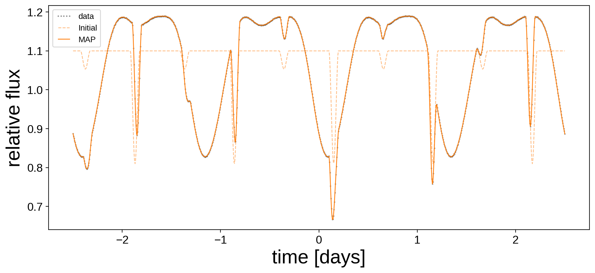
Not bad! Here are the best fit surface maps:

map = starry.Map(ydeg=A["ydeg"])
map.inc = map_soln["A_inc"]
map.amp = map_soln["A_amp"]
map[1:, :] = map_soln["pri_y"]
map.show(theta=np.linspace(0, 360, 50))

map = starry.Map(ydeg=B["ydeg"])
map.inc = map_soln["B_inc"]
map.amp = map_soln["B_amp"]
map[1:, :] = map_soln["sec_y"]
map.show(theta=np.linspace(0, 360, 50))

Also pretty good! Now the fun part: sampling. Sit tight – this will take several hours.

%%time
with model:
    trace = pm.sample(
        tune=2000,
        draws=2500,
        start=map_soln,
        chains=4,
        step=xo.get_dense_nuts_step(target_accept=0.9),
    )

Multiprocess sampling (4 chains in 4 jobs)
NUTS: [sec_y, B_t0, B_porb, B_prot, B_m, B_r, B_amp, B_inc, pri_y, A_prot, A_m, A_r, A_amp, A_inc]
Sampling 4 chains, 308 divergences: 100%|██████████| 18000/18000 [16:27:49<00:00,  3.29s/draws]
There were 68 divergences after tuning. Increase `target_accept` or reparameterize.
There were 80 divergences after tuning. Increase `target_accept` or reparameterize.
There were 79 divergences after tuning. Increase `target_accept` or reparameterize.
There were 81 divergences after tuning. Increase `target_accept` or reparameterize.
The number of effective samples is smaller than 10% for some parameters.

CPU times: user 4h 15min 40s, sys: 21min 47s, total: 4h 37min 27s
Wall time: 16h 29min 28s

That took a very long time. Let’s check the diagnostics:

var_names_A = ["A_m", "A_r", "A_prot", "A_inc", "A_amp"]
var_names_B = ["B_m", "B_r", "B_porb", "B_prot", "B_inc", "B_t0", "B_amp"]
display(pm.summary(trace, var_names=var_names_A + var_names_B))

	mean	sd	hpd_3%	hpd_97%	mcse_mean	mcse_sd	ess_mean	ess_sd	ess_bulk	ess_tail	r_hat
A_m	1.045	0.098	0.867	1.234	0.001	0.001	4291.0	4291.0	4328.0	4468.0	1.00
A_r	1.025	0.029	0.971	1.080	0.000	0.000	3565.0	3545.0	3550.0	5055.0	1.00
A_prot	1.250	0.000	1.250	1.250	0.000	0.000	8705.0	8705.0	8718.0	6825.0	1.00
A_inc	81.211	0.601	80.129	82.380	0.019	0.013	1004.0	1004.0	1008.0	1623.0	1.00
A_amp	1.004	0.021	0.964	1.045	0.001	0.000	1425.0	1416.0	1435.0	2161.0	1.00
B_m	0.701	0.096	0.518	0.876	0.002	0.001	3112.0	3112.0	3105.0	2684.0	1.00
B_r	0.686	0.022	0.646	0.727	0.000	0.000	2528.0	2528.0	2527.0	5394.0	1.00
B_porb	1.000	0.000	1.000	1.000	0.000	0.000	1843.0	1843.0	1850.0	3330.0	1.00
B_prot	0.625	0.000	0.625	0.625	0.000	0.000	7695.0	7695.0	7832.0	5981.0	1.00
B_inc	80.037	0.260	79.541	80.496	0.008	0.006	1047.0	1047.0	1050.0	1806.0	1.01
B_t0	0.150	0.000	0.150	0.150	0.000	0.000	1671.0	1671.0	1673.0	3382.0	1.00
B_amp	0.089	0.006	0.078	0.101	0.000	0.000	777.0	773.0	792.0	1006.0	1.01

They’re not great. The inclination of the primary A_inc and the time of transit B_t0 have fewer than 200 effective samples. We should run the chain for much longer (or reparametrize). But let’s go ahead and plot the posteriors anyways.

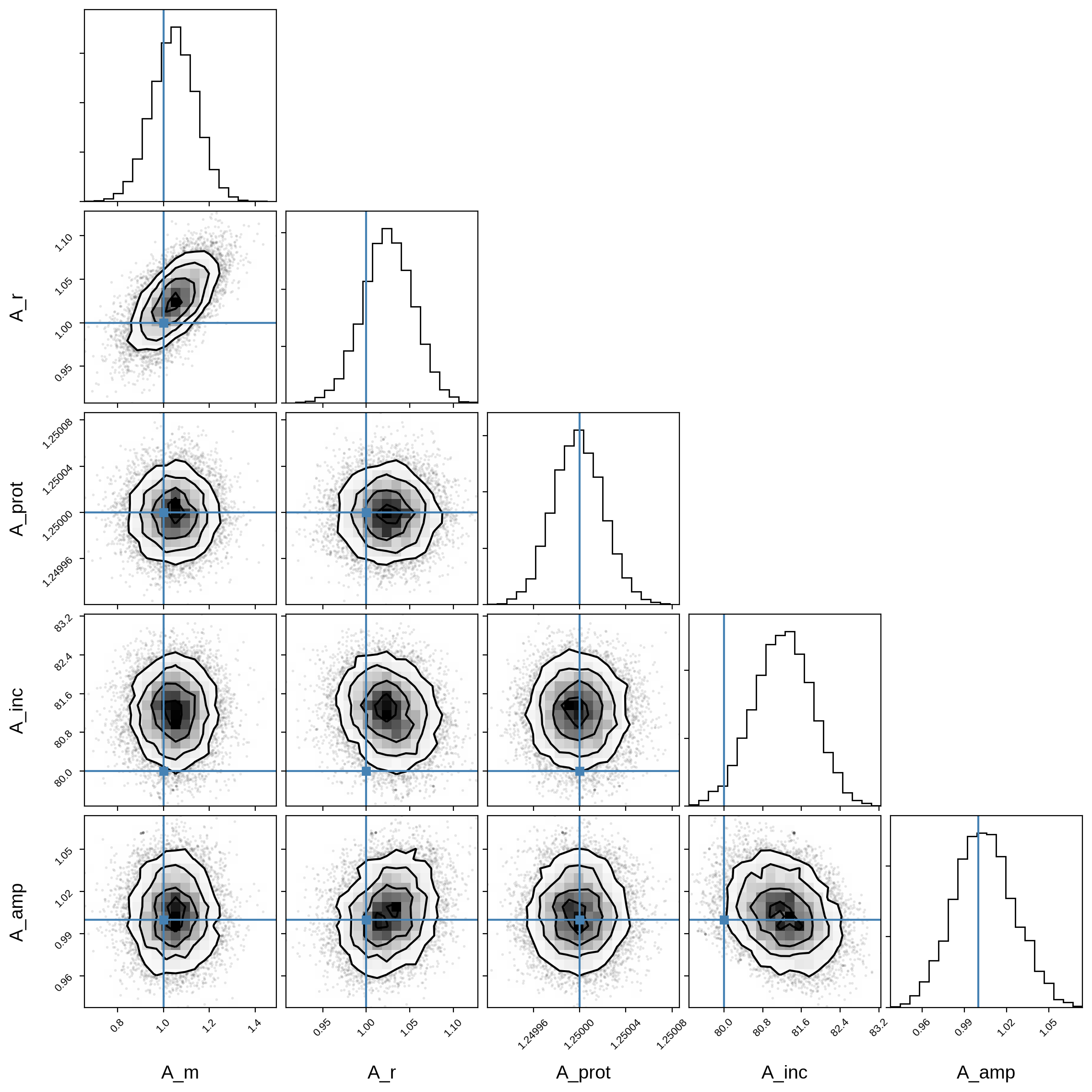
Here’s the corner plot for the posteriors of the primary orbital parameters:

truths_A = [A["m"], A["r"], A["prot"], A["inc"], A["amp"]]
samples_A = pm.trace_to_dataframe(trace, varnames=var_names_A)
corner(samples_A, truths=truths_A);

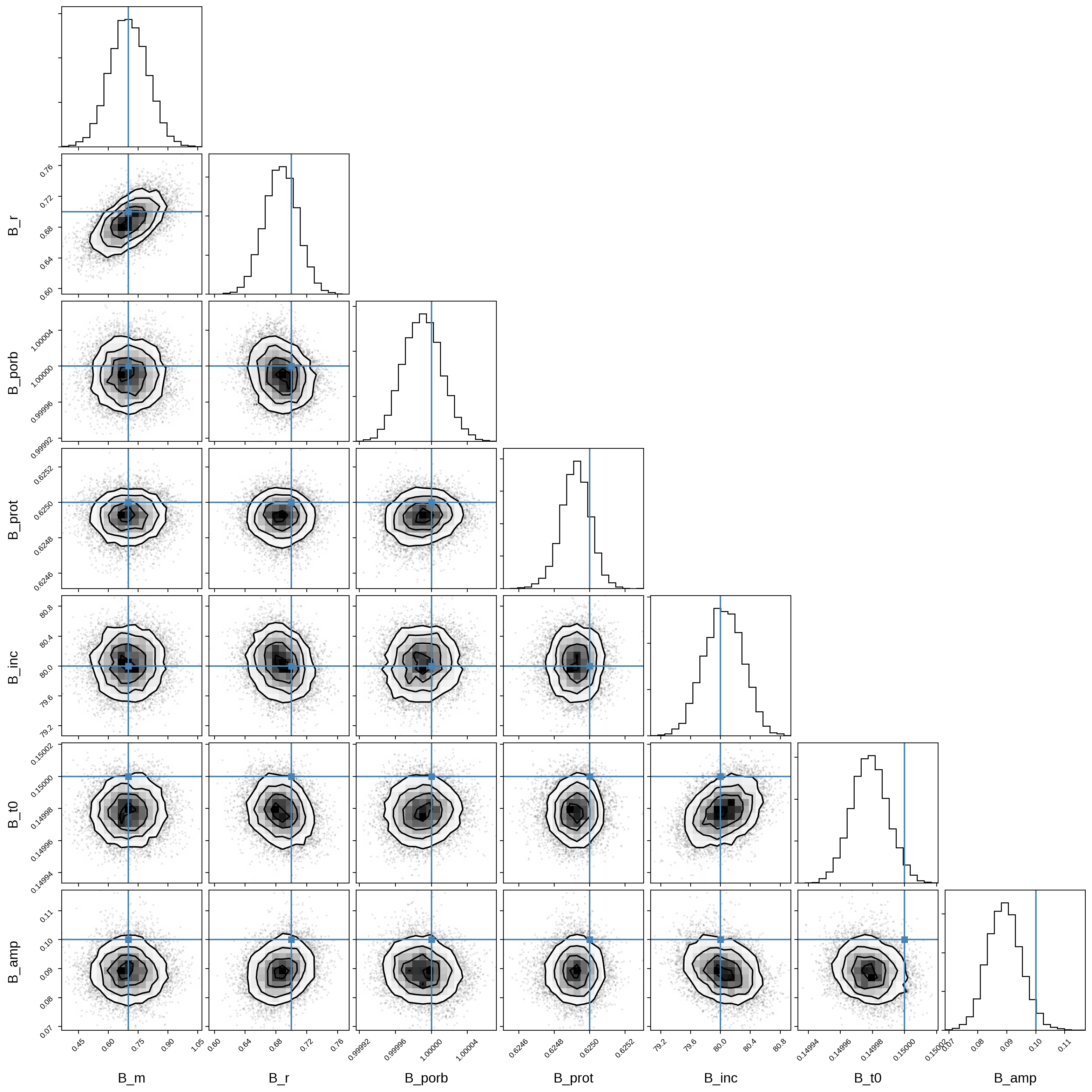
And here’s that same plot for the secondary orbital parameters:

truths_B = [B["m"], B["r"], B["porb"], B["prot"], B["inc"], B["t0"], B["amp"]]
samples_B = pm.trace_to_dataframe(trace, varnames=var_names_B)
corner(samples_B, truths=truths_B);

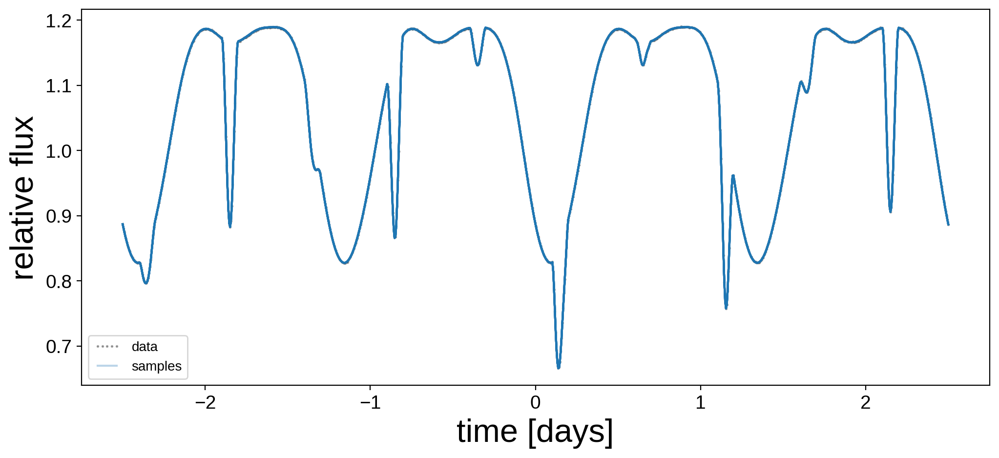
Let’s plot the model for 24 random samples from the chain. Note that the lines are so close together that they’re indistinguishable!

plt.figure(figsize=(12, 5))
plt.plot(t, flux, "k.", alpha=0.3, ms=2, label="data")
label = "samples"
for i in np.random.choice(range(len(trace["flux_model"])), 24):
    plt.plot(t, trace["flux_model"][i], "C0-", alpha=0.3, label=label)
    label = None
plt.legend(fontsize=10, numpoints=5)
plt.xlabel("time [days]", fontsize=24)
plt.ylabel("relative flux", fontsize=24);

Let’s compare the mean map and a random sample to the true map for each star:

# Random sample
np.random.seed(0)
i = np.random.randint(len(trace["pri_y"]))

map = starry.Map(ydeg=A["ydeg"])
map.amp = np.mean(trace["A_amp"])
map[1:, :] = np.mean(trace["pri_y"], axis=0)
pri_mu = map.render(projection="rect").eval()
map.amp = trace["A_amp"][i]
map[1:, :] = trace["pri_y"][i]
pri_draw = map.render(projection="rect").eval()
map.amp = A["amp"]
map[1:, :] = A["y"]
pri_true = map.render(projection="rect").eval()

map = starry.Map(ydeg=B["ydeg"])
map.amp = np.mean(trace["B_amp"])
map[1:, :] = np.mean(trace["sec_y"], axis=0)
sec_mu = map.render(projection="rect").eval()
map.amp = trace["B_amp"][i]
map[1:, :] = trace["sec_y"][i]
sec_draw = map.render(projection="rect").eval()
map.amp = B["amp"]
map[1:, :] = B["y"]
sec_true = map.render(projection="rect").eval()

fig, ax = plt.subplots(3, 2, figsize=(8, 7))
ax[0, 0].imshow(
    pri_true,
    origin="lower",
    extent=(-180, 180, -90, 90),
    cmap="plasma",
    vmin=0,
    vmax=0.4,
)
ax[1, 0].imshow(
    pri_mu,
    origin="lower",
    extent=(-180, 180, -90, 90),
    cmap="plasma",
    vmin=0,
    vmax=0.4,
)
ax[2, 0].imshow(
    pri_draw,
    origin="lower",
    extent=(-180, 180, -90, 90),
    cmap="plasma",
    vmin=0,
    vmax=0.4,
)
ax[0, 1].imshow(
    sec_true,
    origin="lower",
    extent=(-180, 180, -90, 90),
    cmap="plasma",
    vmin=0,
    vmax=0.04,
)
ax[1, 1].imshow(
    sec_mu,
    origin="lower",
    extent=(-180, 180, -90, 90),
    cmap="plasma",
    vmin=0,
    vmax=0.04,
)
ax[2, 1].imshow(
    sec_draw,
    origin="lower",
    extent=(-180, 180, -90, 90),
    cmap="plasma",
    vmin=0,
    vmax=0.04,
)
ax[0, 0].set_title("primary")
ax[0, 1].set_title("secondary")
ax[0, 0].set_ylabel("true", rotation=0, labelpad=20)
ax[1, 0].set_ylabel("mean", rotation=0, labelpad=20)
ax[2, 0].set_ylabel("draw", rotation=0, labelpad=20);

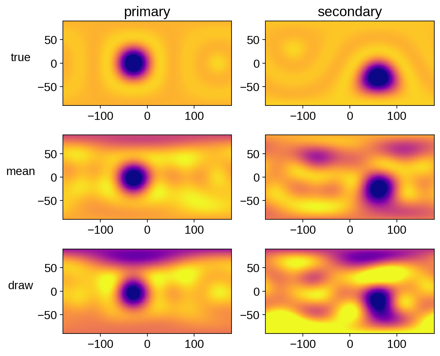
That actually looks pretty good. But keep in mind that we really should have run our chain longer.

However, there is a much better way of doing what we did here. We can combine pymc3 with the linearity of the starry model to come up with a much more efficient way of sampling the posterior. We do that in the next and final notebook of the series.