everest-stats - De-trending Statistics

The everest-stats command accepts several options, which we list below.

season	The season number. For K2, this is the campaign number. Note that fractional seasons are allowed (i.e., 6.0). Default is 0
model	The everest model name. Default nPLD
compare_to	The everest model or pipeline to compare against. Default everest1
-m mission	The mission name (k2 | kepler | tess). Default k2
-s	Plot the short cadence versus long cadence CDPP statistics. If no campaign is specified, shows all campaigns
-p	Plot the CDPP comparison for all confirmed planet hosts
-i	Plot the transit injection/recovery results.

If no flags are specified, everest-stats shows several plots for a given season, comparing everest to a different PLD model or a different mission pipeline. For K2, running

everest-stats 6 nPLD k2sff

produces the following plot:

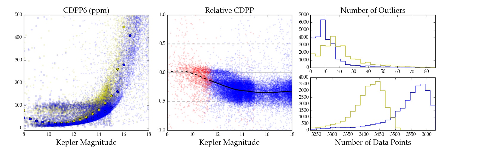
On the left is the CDPP as a function of Kepler magnitude for all stars in campaign 6, de-trended with nPLD (blue dots) and the k2sff pipeline (yellow dots). The median CDPP is indicated by the circles.

In the center is the normalized relative CDPP, given by

Negative values correspond to lower CDPP in the nPLD light curves. Blue dots are unsaturated stars and red dots are saturated stars; the median relative CDPP is indicated by the black lines (solid for unsaturated, dashed for saturated).

On the right we show histograms for the number of outliers (top) and the total number of data points (bottom) for each pipeline.

All points in the first two plots are clickable. Clicking on them will bring up the DVS plots for both pipelines/models for easy comparison.

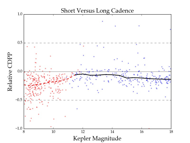
Short Cadence

The -s option allows users to view a comparison between the short cadence and long cadence de-trended light curves. As usual, we plot the normalized relative CDPP. As before, points are clickable and bring up the DVS plots for both the short and long cadence light curves.

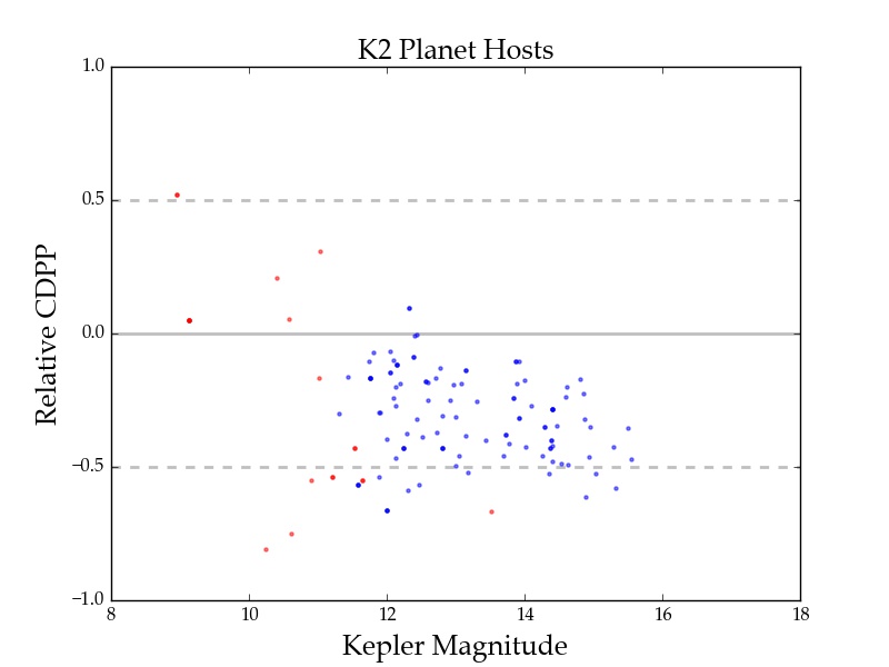
Planets

The -p option allows users to view the statistics for only the confirmed planet hosts. Below is a figure comparing everest to k2sff:

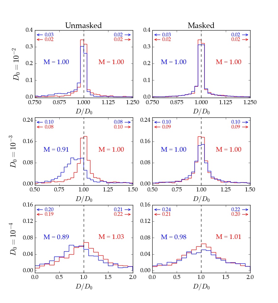
Injections

The -i option plots the results of transit injection/recovery tests. See Figure 6 in Luger et al. (2016) for more information.

Note

For K2, only campaign 6.0 is available. For other campaigns, the user must run the transit injections themselves. See Transit injection.