Note
This tutorial was generated from a Jupyter notebook that can be downloaded here.
A simple exoplanet system
Here we’ll discuss how to instantiate an exoplanet system and compute its full light curve. Currently, all orbital stuff lives in the starry.kepler module, which implements a simple Keplerian solver using the exoplanet package. This works for systems of exoplanets orbiting stars, moons orbiting planets, and binary star systems. Keep in mind, however, that the primary object is assumed to sit at the origin, and the secondary objects are assumed to be massless. A more flexible N-body
solver using rebound is in the works, so stay tuned!
[3]:
import numpy as np
import starry

starry.config.lazy = False
starry.config.quiet = True
Creating a star
Let’s instantiate a Primary object:
[4]:
star = starry.Primary(starry.Map(ydeg=0, udeg=2, amp=1.0), m=1.0, r=1.0, prot=1.0)
The first argument to starry.Primary is a starry.Map instance defining the surface map of the object. We’re giving the star a quadratically limb-darkened (udeg = 2) map with no other spatial features (ydeg = 0). The aplitude amp controls the overall scaling of the intensity of the object and is therefore equal to its luminosity (in arbitrary units).
The starry.Primary class takes additional keywords, including the mass, radius, and rotation period, all of which we set to unity. By default, these are measured in solar units (for the mass and radius) and days (for the periods), though it’s easy to change that. Check out the docs for more details.
Note
Parameters of the surface map (such as ydeg, udeg, and amp) should be passed to the Map object;
all other parameters should be passed directly to the Primary object. You’ll get a warning if you
try to do something like star = starry.Primary(starry.Map(ydeg=0, udeg=2, amp=1.0, m=1.0))
since starry.Map isn’t aware of what a mass is!
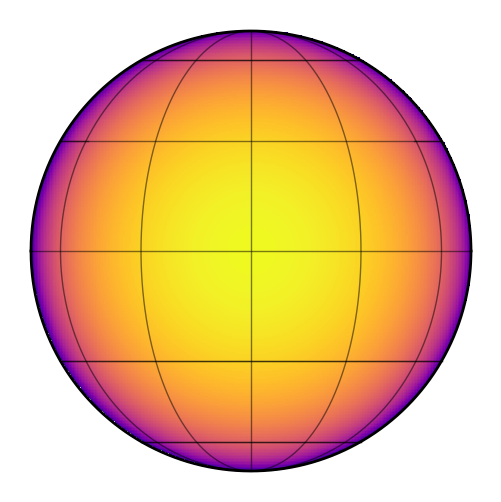
Let’s now set the limb darkening coefficients of the star. Let’s give the stellar map a linear and a quadratic limb-darkening coefficient:
[5]:
star.map[1] = 0.40
star.map[2] = 0.26
Here’s what that looks like:
[6]:
star.map.show()
Creating a planet
Let’s create a (very) hot Jupiter with some interesting properties:
[7]:
planet = starry.kepler.Secondary(
    starry.Map(ydeg=5, amp=5e-3),  # the surface map
    m=0,  # mass in solar masses
    r=0.1,  # radius in solar radii
    porb=1.0,  # orbital period in days
    prot=1.0,  # rotation period in days (synchronous)
    Omega=30,  # longitude of ascending node in degrees
    ecc=0.3,  # eccentricity
    w=30,  # longitude of pericenter in degrees
    t0=0,  # time of transit in days
)
Here we’ve instantiated a planet with a fifth degree surface map, zero mass, a radius that is one-tenth that of the star, a luminosity (amplitude) that is \(5\times 10^{-3}\) times that of the star, an orbital period of 1 day, a rotational period of 1 day, and a bit of an eccentricity.
Note
The default rotational period for objects is infinity, so if you don’t specify prot, the planet’s surface
map will not rotate as the planet orbits the star and there will be no phase curve variation. For planets whose
emission tracks the star (i.e., a hot Jupiter with a hotspot) set prot=porb. Also note that the default
amplitude and mass are both unity, so make sure to change those as well if you don’t want a planet that’s as
bright and as massive as its star!
There are a bunch of other settings related to the orbit, so check out the docs for those. The next thing we get to do is specify the planet’s map. For simplicity, let’s just create a random one:
[8]:
np.random.seed(123)
planet.map[1:, :] = 0.01 * np.random.randn(planet.map.Ny - 1)
[9]:
planet.map.show()
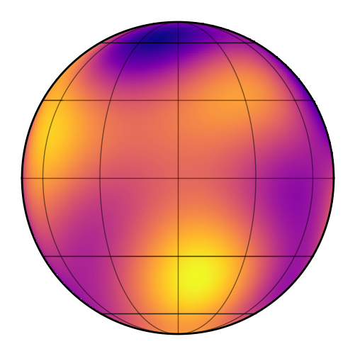
Note that when instantiating a map for a starry.kepler.Secondary instance, the map is defined as it would appear at the reference time, t0. That’s also the time of transit. Quite often we’re interested in the side of the planet that faces the star during secondary eclipse (since that’s what we’re able to map!). In that case, we can specify the initial rotational phase of the planet (when t=t0) to be \(180^\circ\):
[10]:
planet.theta0 = 180
The image above now corresponds to the side of the planet visible during (or near) secondary eclipse, assuming it’s synchronously rotation. Check out the viewing geometry tutorial for more information.
Now, it’s probably a good idea to ensure we didn’t end up with negative specific intensity anywhere:
[11]:
planet.map.minimize()
[11]:
(32.77869170732118, -159.21879080507742, 0.0012465984320517332)
This routine performs gradient descent to try to find the global minimum of the map, and returns the latitude, longitude, and value of the intensity at the minimum. The intensity is positive, so we’re good to go.
Creating a system
Now that we have a star and a planet, we can instantiate a planetary system:
[12]:
system = starry.System(star, planet)
The first argument to a starry.System call is a Primary object, followed by any number of Secondary objects.
There are some other system attributes you can set–notably an exposure time (texp)–if the exposure time of your data is long enough to affect the light curve shape. Check out the docs for more information.
Computing light curves
We’re ready to compute the full system light curve:
[14]:
%%time
time = np.linspace(-0.25, 3.25, 10000)
flux_system = system.flux(time)
CPU times: user 27.6 ms, sys: 0 ns, total: 27.6 ms
Wall time: 27.2 ms
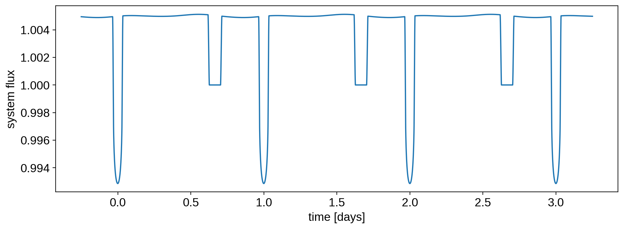
Cool – starry computed 10,000 cadences in a few tens of ms. Let’s check it out:
[15]:
plt.plot(time, flux_system)
plt.xlabel("time [days]")
plt.ylabel("system flux");
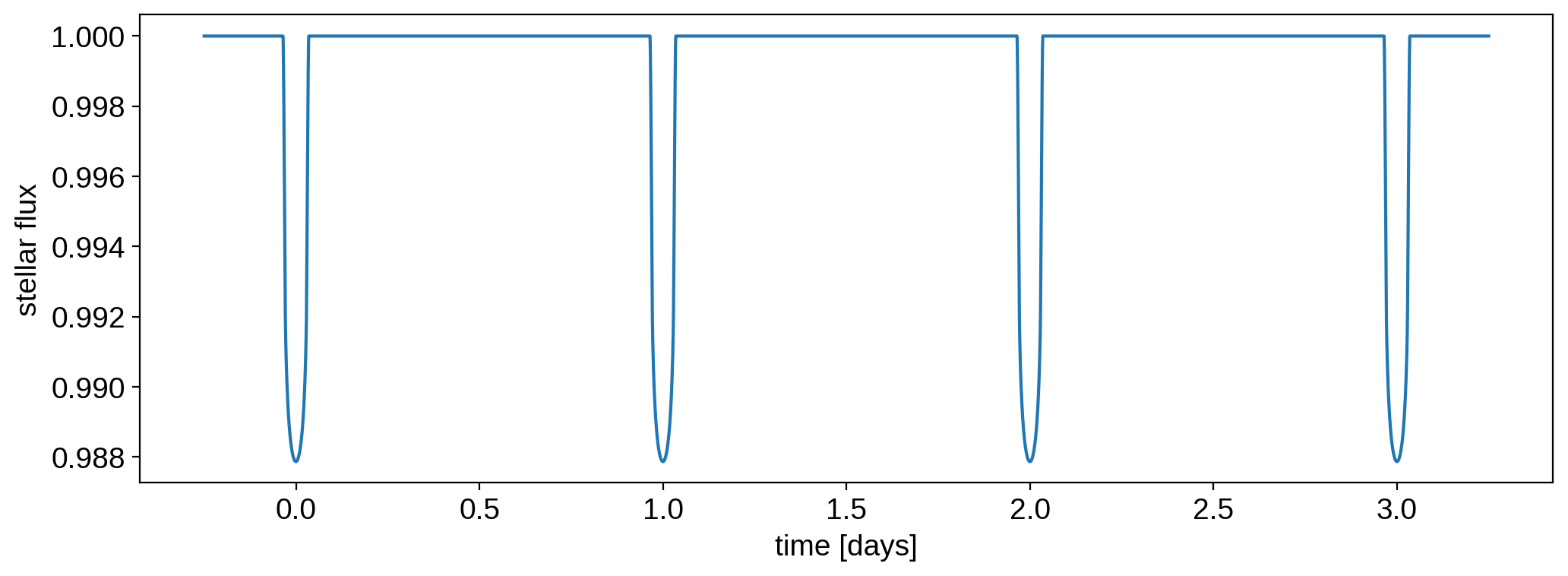
We can also plot the stellar and planetary light curves individually:
[16]:
flux_star, flux_planet = system.flux(time, total=False)
[17]:
plt.plot(time, flux_star)
plt.xlabel("time [days]")
plt.ylabel("stellar flux");
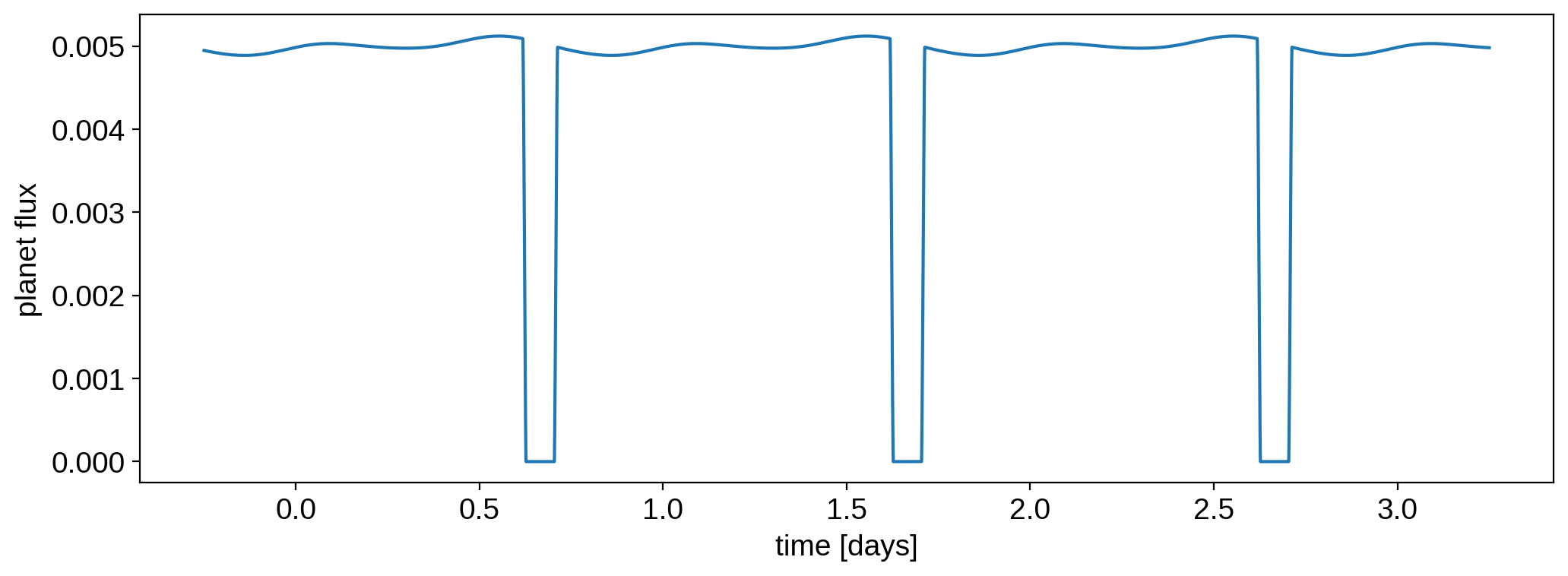
[18]:
plt.plot(time, flux_planet)
plt.xlabel("time [days]")
plt.ylabel("planet flux");
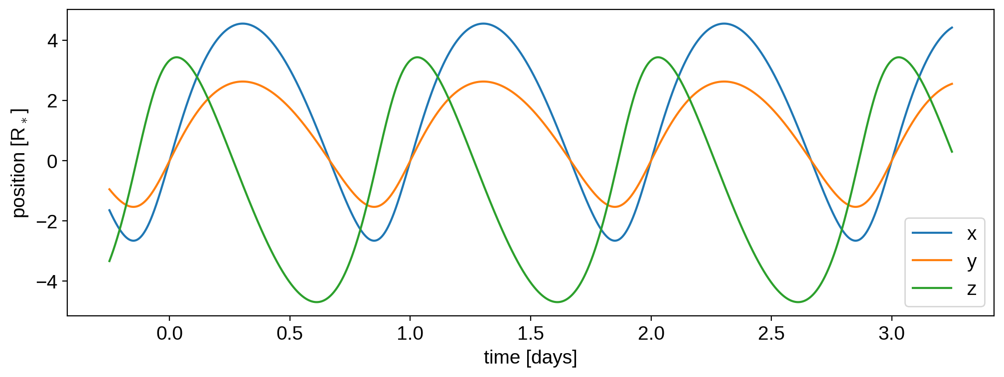
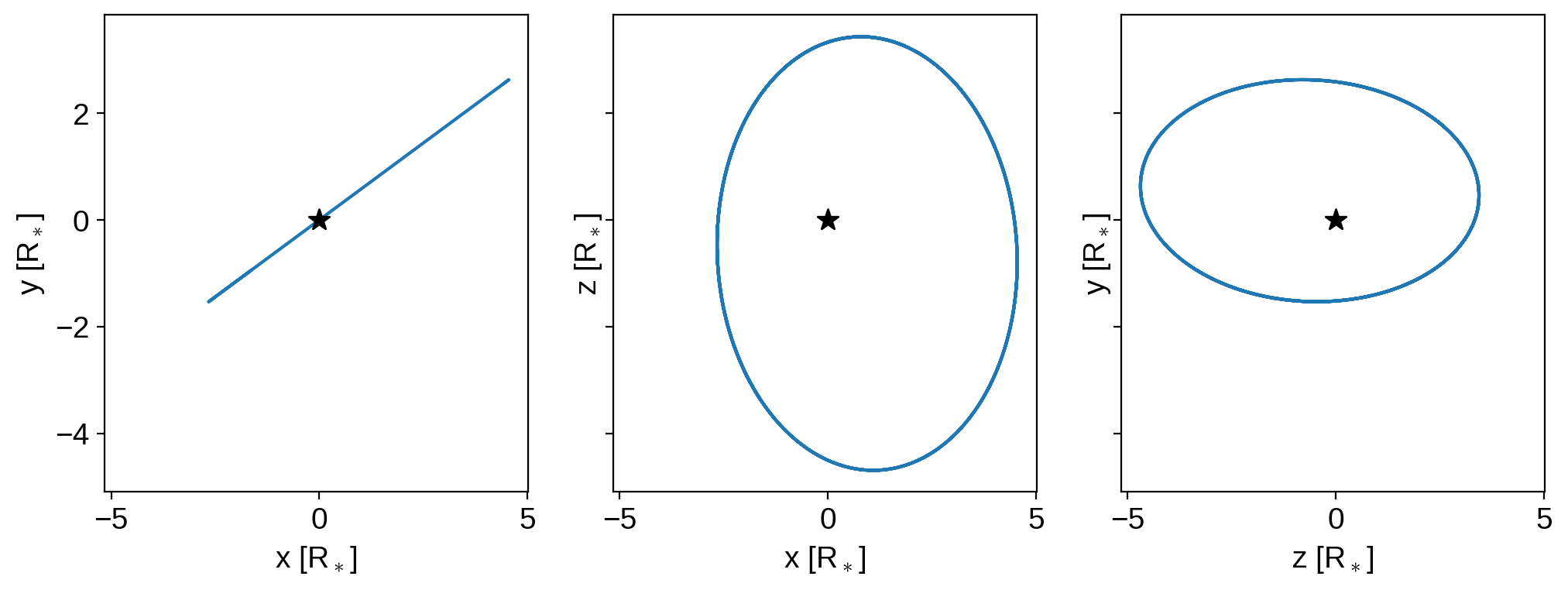
And, just for fun, the planet’s orbit (the sky plane is the \(xy\) plane, with \(y\) pointing up and \(x\) pointing to the right; \(z\) points toward the observer):
[19]:
x, y, z = system.position(time)
The variables \(x\), \(y\), and \(z\) now contain two elements: the position of the star (index 0) and the position of the planet (index 1). Let’s plot the planet’s orbit:
[20]:
plt.plot(time, x[1], label="x")
plt.plot(time, y[1], label="y")
plt.plot(time, z[1], label="z")
plt.ylabel("position [R$_*$]")
plt.xlabel("time [days]")
plt.legend()

fig, ax = plt.subplots(1, 3, sharex=True, sharey=True)
ax[0].plot(x[1], y[1])
ax[1].plot(x[1], z[1])
ax[2].plot(z[1], y[1])
for n in [0, 1, 2]:
    ax[n].scatter(0, 0, marker="*", color="k", s=100, zorder=10)
ax[0].set_xlabel(r"x [R$_*$]")
ax[0].set_ylabel(r"y [R$_*$]")
ax[1].set_xlabel(r"x [R$_*$]")
ax[1].set_ylabel(r"z [R$_*$]")
ax[2].set_xlabel(r"z [R$_*$]")
ax[2].set_ylabel(r"y [R$_*$]");
We can also animate the orbit. We’ll make the planet a little bigger for this visualization:
[21]:
planet.r = 0.33
system.show(t=np.linspace(0, 1, 50), window_pad=4, figsize=(8, 8))
Note
A keen eye might note that the planet’s axis of rotation points up, even though the orbital plane is inclined
(because planet.Omega = 30). If you want the planet’s axis of rotation to be parallel to its orbital axis,
you need to explicitly tell that to starry, since by default the axis of the map points up on the sky.
To do this, set the map’s obliquity equal to the orbital obliquity: planet.map.obl = 30. See the
tutorial on orbital orientation for more information.
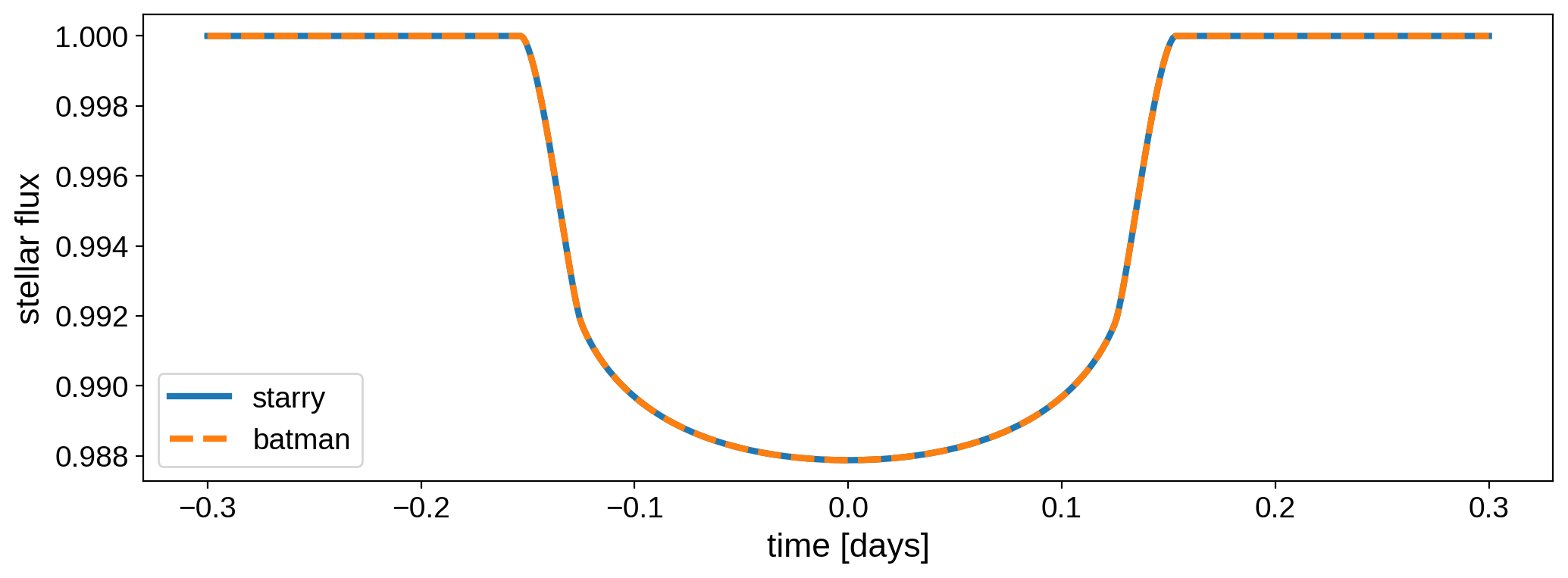
Comparison to batman
One last thing we can do is compare a simple transit calculation to what we’d get with the batman code (Kreidberg 2015), a widely used and well-tested light curve tool.
First, let’s define all the system parameters:
[22]:
u1 = 0.4  # Stellar linear limb darkening coefficient
u2 = 0.26  # Stellar quadratic limb darkening coefficient
rplanet = 0.1  # Planet radius in units of stellar radius
inc = 89.95  # Planet orbital inclination
per = 50  # Planet orbital period in days
mstar = 1  # Stellar mass in Msun
rstar = 1  # Stellar radius in Rsun
a = (per ** 2 * starry._constants.G_grav * mstar / (4 * np.pi ** 2)) ** (
    1.0 / 3.0
)  # semi-major axis in Rsun
We’ll evaluate the light curve on the following time grid:
[23]:
npts = 500
time = np.linspace(-0.3, 0.3, npts)
Let’s evaluate the starry light curve for this system:
[24]:
# Instantiate the star
star = starry.Primary(starry.Map(udeg=2))
star.map[1] = u1
star.map[2] = u2

# Instantiate the planet
planet = starry.kepler.Secondary(starry.Map(amp=0), m=0, porb=per, inc=inc, r=rplanet)

# Instantiate the system
system = starry.System(star, planet)

# Compute and store the light curve
flux_starry = system.flux(time)
And now the batman light curve:
[25]:
import batman

params = batman.TransitParams()
params.limb_dark = "quadratic"
params.u = [u1, u2]
params.t0 = 0.0
params.ecc = 0.0
params.w = 90.0
params.rp = rplanet
params.a = a
params.per = per
params.inc = inc
m = batman.TransitModel(params, time)
flux_batman = m.light_curve(params)
Let’s plot the two light curves:
[26]:
plt.plot(time, flux_starry, label="starry", lw=3)
plt.plot(time, flux_batman, "--", label="batman", lw=3)
plt.xlabel("time [days]", fontsize=16)
plt.ylabel("stellar flux", fontsize=16)
plt.legend();
Here is the difference between the two models:
[27]:
plt.plot(time, flux_starry - flux_batman)
plt.xlabel("time [days]")
plt.ylabel("residuals");
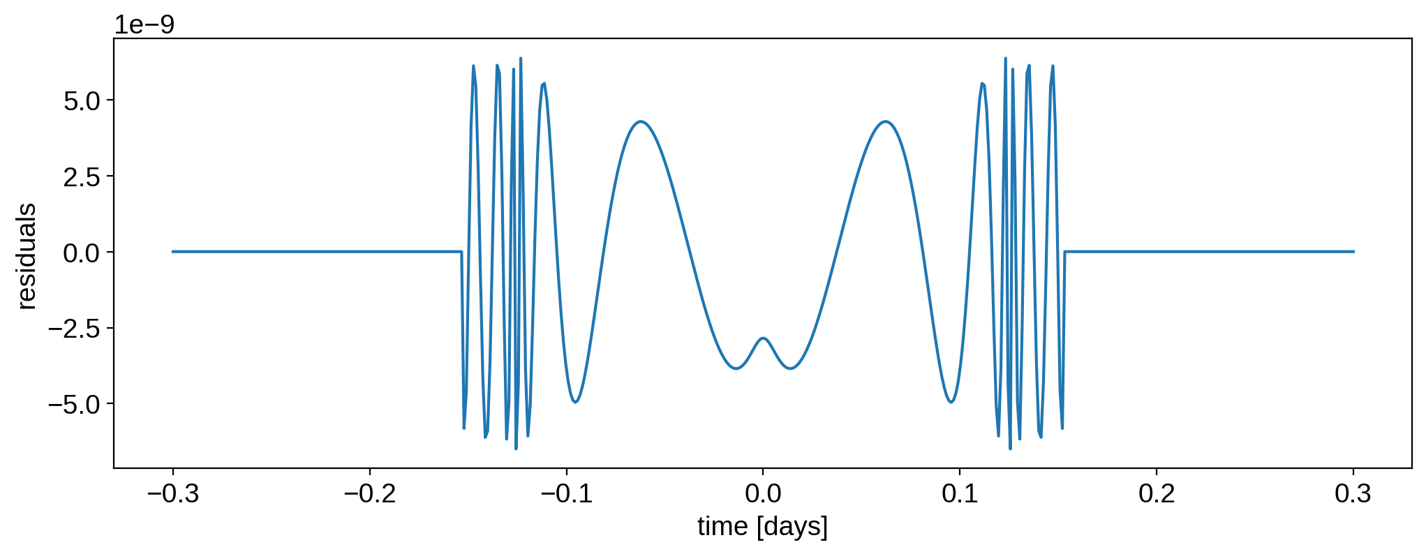
It’s on the order of a few parts per billion, which is quite small. The oscillations are due to the fact that batman uses Hasting’s approximation to compute the elliptic integrals, which is slightly faster but leads to small errors. In practice, however, the two models are equivalent for exoplanet transit modeling.